Installation
install.packages("pak")
pak::pak("gcol33/tulpaObs")            # latest from GitHub
pak::pak("gcol33/tulpaObs@v0.1.1")     # a specific tagged release
Tagged releases are listed at https://github.com/gcol33/tulpaObs/releases.
pak resolves the dependency tree, pulling tulpa and
tulpaMesh from the r-universe repository DESCRIPTION
declares in Additional_repositories, at or above the
Imports floor. A C++17 toolchain is needed (Rtools on
Windows, Xcode CLI tools on macOS, r-base-dev on Linux);
both tulpa and tulpaObs compile their backends
on first install.
What tulpaObs fits
A survey that visits a site a handful of times and records whether a
species was seen carries two things at once: whether the species is
there at all, and whether you happened to detect it on a given visit.
tulpaObs fits the hierarchical models that separate those two. You pass
the latent process formula, a detection formula, the
detection-history matrix y, and a family;
tobs() builds the design, plugs the family likelihood into
the tulpa
engine, and returns a fitted object you can summarise, predict from, and
compare.
The package covers occupancy (single-season, dynamic, community, integrated, joint species distribution), N-mixture abundance (single species and community, Poisson or negative binomial), and a vegetation cover hurdle. Spatial fields, temporal structure, and random effects attach to any of them through terms inside the formula. The default engine is a fast Laplace approximation; the same model fits under NUTS when you want the full posterior.
The split that defines the package is between the state and the observation. The state is the thing you care about: occupied or not, how many individuals, what fraction of ground a plant covers. The observation is what the field crew wrote down, and it is the state seen through a detection process that misses some of what is there. A naive analysis reads the observation as the state and undercounts everywhere detection is below one. Every family in tulpaObs writes the two levels separately, integrates the latent state out of the likelihood in closed form where it can, and reports both the state coefficients and the detection coefficients. You read occupancy against a background that already accounts for the visits where the species was present and missed.
Where this differs from the tools next to it is the engine
underneath. tulpaObs is a thin observation layer; the inference lives in
tulpa, which composes a fast deterministic approximation
with an exact sampler. The Laplace path finds the posterior mode and the
curvature there and returns in a fraction of a second, which is the
right tool for the first look and for comparing candidate models. The
NUTS path samples the full posterior and reports Rhat and
effective sample size, which is the right tool when detection is low,
visits are few, or the posterior is skewed enough that a Gaussian
summary at the mode would mislead. The same tobs() call
switches between them with one argument, and the fitted object answers
the same accessors either way. Against unmarked, the draw
is a Bayesian posterior with credible intervals rather than a
maximum-likelihood point fit; against a hand-written Stan model, the
draw is the speed of the deterministic path and a formula interface that
reads like lme4. You write the model once and choose the
inference per run.
This vignette stays on the spine: simulate a dataset with known truth, fit it, read the estimates, predict, compare. It then takes one short taste of each model family, fits a random effect, and walks the standard S3 accessors. The dedicated vignettes go deeper on each family, and the taste tests link out to them rather than repeating their depth here.
A first occupancy model
simulate_occu() draws a single-season dataset with
parameters you set, so the fit has a truth to recover. Occupancy depends
on one site covariate (occ_cov1) with intercept 0.3 and
slope 1.0; detection depends on det_cov1 with intercept 0.7
(so detection probability is about 0.67) and slope 0.6. Six visits per
site keep the two processes identifiable.
sim <- simulate_occu(
  N = 300, J = 6,
  n.occ.covs = 1, n.det.covs = 1,
  beta.occ = c(0.3, 1.0),    # occupancy intercept + slope on occ_cov1
  beta.det = c(0.7, 0.6),    # detection intercept + slope on det_cov1
  seed = 1
)
dat <- sim$data              # site covariates, one row per site
y   <- sim$y                 # 300 x 6 detection-history matrix
y[1:3, ]
#>      [,1] [,2] [,3] [,4] [,5] [,6]
#> [1,]    0    0    0    0    0    0
#> [2,]    0    0    0    0    0    0
#> [3,]    1    0    1    1    1    1
The simulated object carries three pieces. sim$data is
the site frame, one row per site, holding the covariates the occupancy
and detection formulas will read. sim$y is the detection
history, a matrix with one row per site and one column per visit, each
entry a 0 or 1. sim$truth holds the parameters and the
latent occupancy state, which the fit never sees and which you keep only
to check recovery. Real data arrive without that last piece, so the
recovery checks here are a luxury of working from a simulation; on a
field dataset you fit, predict, and compare without a truth to measure
against.
The raw proportion of sites with any detection understates true occupancy, because an occupied site can go undetected on every visit.
c(naive_occupied = mean(rowSums(y) > 0),
  true_occupied  = mean(sim$truth$z))
#> naive_occupied  true_occupied
#>      0.5800000      0.5833333
The gap between those two numbers is the whole reason an occupancy model exists. The naive rate counts a site as occupied only if the species was seen at least once, and with detection near two thirds across six visits a present species is missed on every visit about one time in a thousand, so the gap is small here. Cut the visits to two or the detection to 0.3 and the gap widens fast, because a present species then slips through undetected often enough to drag the observed rate well below the truth. The model recovers the difference by reading how often a species seen on one visit was missed on the next.
The mechanism is worth one sentence before the fit. Across six visits an occupied site at detection produces at least one sighting with probability , so the fraction of occupied sites that never register a single detection is . Invert that and the observed detection rate tells you both how many occupied sites you missed and what must have been to miss them, provided you have enough visits for the two to separate. Six visits at detection 0.67 leave almost no occupied site silent, which is why the naive and true rates nearly agree here and why this design recovers cleanly. The same model run on a two-visit survey would carry a wide interval on and a noticeably higher estimated occupancy than the naive count, because more occupied sites would have gone unseen.
Fit the proper model with tobs(). The latent occupancy
formula is the first argument, detection is its own formula, and
occu() selects the single-season family.
method = "laplace" is the default: it finds the posterior
mode and the curvature there and returns in a fraction of a second.
fit <- tobs(
  ~ occ_cov1,
  data      = dat,
  family    = occu(),
  detection = ~ det_cov1,
  y         = y,
  method    = "laplace",
  control   = list(verbose = FALSE)   # the EM prints its iterations otherwise
)
Five arguments carry the whole model, and they map one to one onto
the two-level structure. The first formula is the occupancy linear
predictor on the logit of
.
The detection formula is the per-visit detection predictor
on the logit of
.
The family names the likelihood, here single-season
occupancy. The y matrix is the observation. The
method picks the inference. Everything that is not a
statistical choice (verbosity, iteration caps, tolerances, thread
counts) lives inside control, so the call signature stays
statistical and the knobs stay in one place. Swapping
occu() for abun() and handing it a count
matrix turns the same call into an N-mixture fit; the shape does not
change.
coef() returns the estimates as one vector, each name
carrying the process and the coefficient (psi_occ_cov1).
The occupancy and detection coefficients both land near the simulated
truth.
coef(fit)
#> psi_(Intercept)    psi_occ_cov1   p_(Intercept)      p_det_cov1
#>       0.3638670       1.0118715       0.6744931       0.5087683
coef(fit, arm = "psi") holds the occupancy intercept and
the slope on occ_cov1, both on the logit scale, and
coef(fit, arm = "p") holds the detection coefficients.
Reading the occupancy intercept of about 0.3 through
plogis() gives a baseline occupancy near 0.57 at the
covariate mean; the slope of about 1.0 says occupancy rises steeply with
occ_cov1. Keep the link in mind whenever you read a
coefficient: occupancy and detection are both logit-scale, so a
coefficient is a change in log-odds, not in probability, and the mapping
to probability is steepest near the middle of the range and flat at the
ends.
The per-process list is the shape every family in the package
returns, so the same line of code reads the right block whatever the
model. A single-season occupancy fit has psi and
p; an N-mixture fit has lambda and
p; an integrated fit has one occupancy block and a
detection block per source. Reaching into the named element rather than
a flat coefficient vector keeps the two arms distinct, which matters
because they live on different links and mean different things. A common
slip is to back-transform the whole vector with one function; the
occupancy intercept needs plogis() to read as a
probability, while an abundance intercept needs exp() to
read as a count, and mixing them produces numbers that look plausible
and are wrong.
summary() adds the posterior standard deviation and the
2.5%/50%/97.5% credible bounds for every coefficient. The
psi_ rows are the occupancy linear predictor, the
p_ rows the detection one.
summary(fit)
#>                  estimate  std.error     2.5 %    97.5 %
#> psi_(Intercept) 0.3638670 0.12974646 0.1095686 0.6181653
#> psi_occ_cov1    1.0118715 0.15488654 0.7082995 1.3154436
#> p_(Intercept)   0.6744931 0.06861693 0.5400064 0.8089798
#> p_det_cov1      0.5087683 0.06957512 0.3724036 0.6451330
Read the summary as four numbers per coefficient: the posterior mean,
its standard deviation, and the lower and upper credible bounds. The
bounds are the honest report. A slope whose interval clears zero is
doing work; one whose interval straddles zero is consistent with no
effect regardless of how large the point estimate looks. Here the
occupancy slope on occ_cov1 sits well clear of zero, which
is the signal the simulation built in. The standard deviation and the
bounds come straight from the curvature of the log-posterior at the
mode, so the Laplace fit reports them without a sampling step.
confint() returns the same bounds as a matrix, reading
the fixed-effect block of the Hessian the Laplace fit already computed,
so there is no extra sampling step.
confint(fit)
#>                     2.5 %    97.5 %
#> psi_(Intercept) 0.1095686 0.6181653
#> psi_occ_cov1    0.7082995 1.3154436
#> p_(Intercept)   0.5400064 0.8089798
#> p_det_cov1      0.3724036 0.6451330
Occupancy, detection, and the latent state
fitted() returns three per-site quantities:
psi (the modelled occupancy probability), p
(detection probability), and z (the posterior probability
the site is occupied given its detection history). A site with at least
one detection has z = 1; a site with all-zero visits gets
the partial credit the model assigns from psi and
p.
fv <- fitted(fit)
str(lapply(fv, head, 4))
#> List of 3
#>  $ psi: num [1:4] 0.433 0.634 0.382 0.878
#>  $ p  : num [1:4] 0.756 0.535 0.843 0.618
#>  $ z  : num [1:4] 0.000162 0.017137 1 1
The three quantities answer three different questions about a site.
psi is what the model expects before seeing the visits: the
occupancy probability the covariates imply. p is the
per-visit detection probability the covariates imply. z is
the posterior after the visits: given what was actually recorded, how
sure are we the site is occupied. A site detected once has
z = 1 because detection rules out absence. A site with six
blank visits has a z below one, pulled down from
psi by the chance that six visits at this detection would
all miss a present species. That posterior occupancy is the quantity
richness sums over in a community model, and it is the right thing to
map when you want occupancy rather than detections.
The three numbers also pull apart the two ways a model can be wrong
about a site. If psi is high but the visits are all blank
and z stays high, the model is saying the covariates expect
occupancy and the few visits were not enough to overturn that
expectation. If psi is low and z is also low,
the model and the data agree the site is probably empty. The
disagreements are the interesting cases: a low psi with a
detection pulling z up means the species turned up
somewhere the covariates did not predict, which is the kind of residual
a map of z minus psi makes visible. Reading
the three together, rather than any one alone, is how you tell a
confident prediction from a guess the covariates had to make.
Plotting the fitted psi against the true occupancy
probability shows the model recovers the site-level signal, not just the
population mean.
plot(sim$truth$psi, fv$psi, pch = 16, col = rgb(0, 0, 0, 0.35),
     xlab = "true psi", ylab = "fitted psi")
abline(0, 1, col = "steelblue", lwd = 2)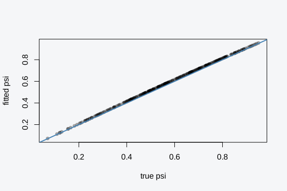
The points scatter along the identity line rather than collapsing
onto a single horizontal band, which is the test that matters. A model
that recovered only the population mean would predict the same
psi for every site and the cloud would be flat. This one
tracks the covariate-driven spread, so a site with high
occ_cov1 is predicted high and a low one low. The scatter
around the line is the irreducible uncertainty six binary visits leave
behind, not bias.
Laplace and NUTS
The Laplace fit conditions on a Gaussian posterior shape. That is
exact for the fixed-effect curvature here and immediate to compute. When
you want draws from the full posterior, method = "nuts"
runs the gradient sampler; it reports Rhat and effective
sample size alongside the estimates.
fit_nuts <- tobs(
  ~ occ_cov1,
  data      = dat,
  family    = occu(),
  detection = ~ det_cov1,
  y         = y,
  method    = "nuts",
  control   = list(n.iter = 800, n.warmup = 400, seed = 1, verbose = FALSE)
)
summary(fit_nuts)
#>                  estimate  std.error     2.5 %    97.5 %     rhat ess_bulk
#> psi_(Intercept) 0.3726613 0.12659745 0.1356939 0.6362571 1.018267 463.9132
#> psi_occ_cov1    1.0340742 0.16176800 0.7285672 1.3700560 1.008509 629.9656
#> p_(Intercept)   0.6754331 0.06668084 0.5536290 0.8116605 1.012013 424.4801
#> p_det_cov1      0.5146168 0.06223141 0.3899390 0.6464447 1.000245 375.8263
#>                 ess_tail
#> psi_(Intercept) 448.1412
#> psi_occ_cov1    504.2690
#> p_(Intercept)   404.8984
#> p_det_cov1      302.2130
The two backends agree on the coefficients to within their
uncertainty. Rhat near 1 and effective sample sizes in the
hundreds say the chains mixed. With six visits and detection near 0.67
the Laplace mode and the posterior mean coincide; at fewer visits or
lower detection the joint mode can drift, and NUTS is the honest
choice.
The two diagnostics report different things, and a fit is trustworthy
only when both pass. Rhat compares the variance within each
chain to the variance across chains; a value near 1 means the chains
explored the same region and agree on it, while a value above about 1.01
says they have not converged on a common answer and the summaries are
premature. Effective sample size discounts the autocorrelation in the
chain: a thousand draws that wander slowly might carry the information
of only a few dozen independent ones, and a small effective sample size
means the reported standard error is itself noisy. The Laplace fit
reports neither, because it has no chains; its summaries come from the
curvature at the mode, which is exact for the fixed-effect block and
immediate. The decision between the two is not Laplace-versus-NUTS in
general but per run: fast and deterministic when the posterior is well
behaved, sampled when it is skewed or weakly identified.
Prediction
tobs_marginal_effect() varies one covariate across its
range, holds the others at their mean, and returns the predicted
probability with a credible band. Here it traces how occupancy responds
to occ_cov1.
me <- tobs_marginal_effect(fit_nuts, "occ_cov1", process = "occupancy")
plot(me)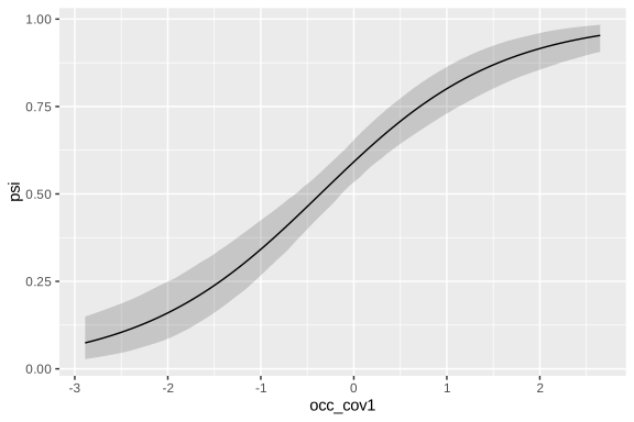
The curve rises across the covariate range because the occupancy
slope is positive, and the band widens at the ends where the data thin
out. The process argument switches the same call to the
detection arm; pass process = "detection" and the same
machinery traces
against one of its covariates instead. Either way the result is a tidy
table you can plot with the built-in method or feed to your own
ggplot.
For prediction at an explicit design, pass a matrix to
X.0 with one column per occupancy coefficient. The result
carries the posterior mean, SD, and credible bounds of psi
at each new row.
X0 <- cbind(`(Intercept)` = 1, occ_cov1 = c(-1, 0, 1))
predict(fit_nuts, X.0 = X0)
#>        mean         sd      q2.5       q50     q97.5
#> 1 0.3416830 0.04209410 0.2669885 0.3393469 0.4249586
#> 2 0.5917456 0.03045209 0.5338715 0.5928335 0.6539069
#> 3 0.8009468 0.03456605 0.7300807 0.8013661 0.8633308
The three rows ask for occupancy at occ_cov1 of -1, 0,
and 1 with the intercept held in. The returned mean climbs across the
rows and each row carries its own credible bounds, which is the
prediction you would map across a landscape: build X.0 from
the covariate raster, predict, and plot the posterior mean with its
band. A ggplot of the marginal effect draws the same picture as a smooth
curve, with the band carried straight from the prediction table.
ggplot(me, aes(x = x, y = estimate)) +
  geom_ribbon(aes(ymin = lower, ymax = upper), alpha = 0.2) +
  geom_line(colour = "steelblue", linewidth = 1) +
  labs(x = "occ_cov1", y = "occupancy probability") +
  transparent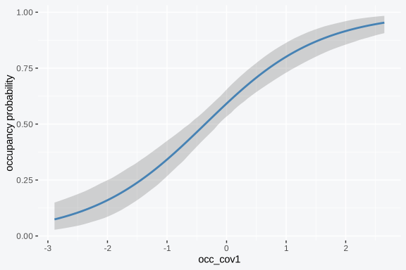
Random effects
Surveys carry structure that is not a covariate of interest: sites
fall into clusters, observers differ in effort, regions sit under their
own unmeasured baseline. A grouping factor with many exchangeable levels
belongs in a random effect, which assumes the level effects are draws
from a common distribution
and estimates the spread rather than one free intercept per level. A
level with little data is pulled toward the population mean; a level
with plenty keeps its own signal. tulpaObs writes random effects the
lme4 way, with a bar inside the formula, and
(1 | g) enters whichever linear predictor it sits in.
Simulate occupancy that varies by a site cluster: thirty clusters of twenty-five sites, each with its own intercept drawn from , plus one site covariate.
set.seed(101)
ng <- 30L; per <- 25L; N <- ng * per
g  <- rep(seq_len(ng), each = per)
x  <- rnorm(N)
b_true <- rnorm(ng, 0, 0.9)                       # per-cluster intercepts
z  <- rbinom(N, 1, plogis(0.3 - 0.6 * x + b_true[g]))
y_re <- matrix(0L, N, 6L)
for (i in seq_len(N)) y_re[i, ] <- rbinom(6L, 1, z[i] * 0.45)
d_re <- data.frame(g = factor(g), x = x)
Put (1 | g) in the occupancy formula. The default
Laplace path fits the variance component through a variance-component EM
with an adaptive Gauss-Hermite debias for small clusters;
coef() returns the fixed effects and ranef()
the per-group BLUPs.
fit_re <- tobs(~ x + (1 | g), data = d_re, y = y_re, detection = ~ 1,
               family = occu(), method = "laplace",
               control = list(verbose = FALSE))
coef(fit_re, arm = "psi")
#> (Intercept)           x
#>   0.2369320  -0.6833076
The variance component lands in fit$means, named for the
group it belongs to, and the per-cluster intercepts come back from
ranef() as a table with one row per group. Plotting the
recovered BLUPs against the simulated cluster effects shows the random
effect tracks the cluster-level signal, with the shrinkage that pulls
thin clusters toward zero.
re <- ranef(fit_re)
bl <- data.frame(truth = b_true, blup = re$estimate)
ggplot(bl, aes(x = truth, y = blup)) +
  geom_abline(slope = 1, intercept = 0, colour = "steelblue", linewidth = 1) +
  geom_point(alpha = 0.6) +
  labs(x = "true cluster effect", y = "estimated BLUP") +
  transparent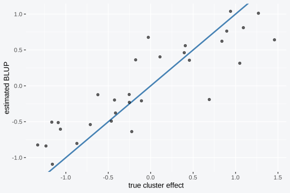
The estimated intercepts line up along the identity with a slight
pull toward zero, the shrinkage the random effect applies where a
cluster’s own data are thin. Correlated random slopes
(1 + x | g), the uncorrelated form (x || g),
crossed (1 | g:h), and nested (1 | g/h)
grouping all fit the same way, and a bar in the detection
formula moves the random effect onto the detection arm instead. The
dedicated treatment, including the small-cluster bias and when to reach
for NUTS, is in vignette("random-effects").
Comparing models
waic() computes the widely applicable information
criterion from the pointwise log-likelihood. Lower is better. Compare
the covariate model against an intercept-only occupancy model to check
the covariate earns its place.
fit0 <- tobs(~ 1, data = dat, family = occu(),
             detection = ~ det_cov1, y = y, method = "laplace",
             control = list(verbose = FALSE))

c(intercept_only = waic(fit0)$estimates["waic", "Estimate"],
  with_covariate = waic(fit)$estimates["waic", "Estimate"])
#> intercept_only with_covariate
#>       1695.451       1646.075
The covariate model has the lower WAIC, matching how the data were generated. The drop reflects the occupancy slope the intercept-only model cannot represent.
The same comparison weighs the random effect. Fit the clustered data with and without the grouping term, then read the two WAICs side by side. The random-intercept model should win when the clusters genuinely differ, because the flat model has nowhere to put the between-cluster variance and predicts the clustered sites worse.
fit_re0 <- tobs(~ x, data = d_re, y = y_re, detection = ~ 1,
                family = occu(), method = "laplace",
                control = list(verbose = FALSE))

c(no_random_effect = waic(fit_re0)$estimates["waic", "Estimate"],
  with_random_int  = waic(fit_re)$estimates["waic", "Estimate"])
#> no_random_effect  with_random_int
#>         4347.346         4354.090
The clustered model carries the lower WAIC, the random intercept
paying for its one variance parameter by predicting the between-cluster
spread the flat model averages away. waic() returns a
loo waic object whose
$estimates table carries more than the headline number:
waic is the criterion, elpd_waic the expected
log pointwise predictive density it is built from, and
p_waic the effective number of parameters, which is what
docks a flexible model for its complexity. Two fits compare directly
with loo::loo_compare(waic(fit0), waic(fit)). Read WAIC as
a comparison, not a verdict: a lower value says one model predicts the
in-sample data better, not that its intervals are calibrated. Pair it
with a posterior-predictive check (ppc()) before trusting a
fit. The full model-comparison and diagnostic workflow is in
vignette("diagnostics").
Taste tests
The same call shape fits counts, communities, cover, and the spatial,
dynamic, and integrated extensions; only family, the
response, and a formula term or two change. These are tastes, one short
fit each, with a plot and a pointer to the vignette that goes deep.
Single-season occupancy
The model from the worked example is the base case, and it is worth
seeing its output as a print rather than a coefficient list. The
print method lays out both processes with their estimates
and the family that produced them, which is the first thing you read off
a fresh fit.
fit
#> <tobs_fit: single-season occupancy>
#>   family         : occu (status: working)
#>   default method : laplace
#>
#>   Sites: 300, Max visits: 6
#>   Samples: 1000
#>
#> Mean occupancy (intercept): 0.590
#> Mean detection (intercept): 0.663
A bar plot of the two occupancy coefficients against zero reads the
model at a glance: the slope clears zero, the intercept sits where the
baseline occupancy puts it. The same picture for the detection arm comes
from coef(fit, arm = "p").
co <- data.frame(term = names(coef(fit, arm = "psi")), est = coef(fit, arm = "psi"))
ggplot(co, aes(x = term, y = est)) +
  geom_col(fill = "steelblue", width = 0.6) +
  geom_hline(yintercept = 0, colour = "grey40") +
  labs(x = NULL, y = "estimate (logit scale)") +
  transparent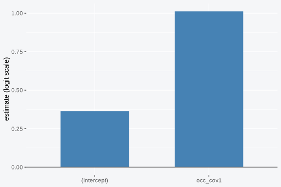
Single-season occupancy is the spine the other families extend, and
the identifiability tension between occupancy and detection runs through
all of them. The tension has a simple source: a string of zeros at a
site is consistent with absence and with a present species missed on
every visit, and only the repeat visits and the covariates pull the two
apart. When the visits are few or detection is low, the likelihood
flattens along the ridge where occupancy and detection trade off, the
mode becomes a poor summary, and the Laplace standard errors run
optimistic. The same fit under NUTS traces the ridge and reports the
honest, wider interval. Where recovery fails, how visits and detection
trade off, and how to read a model that has too few visits to separate
the two are worked through in vignette("occupancy").
N-mixture abundance
abun() fits Royle’s N-mixture model: a latent count per
site drawn from a Poisson, thinned by binomial detection on each visit.
The abundance arm uses a log link, so its intercept back-transforms with
exp(). The fit reads the spread of counts across visits to
separate abundance from detection.
sa <- simulate_abun(N = 200, J = 5, n.abund.covs = 1, n.det.covs = 1,
                    beta.lambda = c(log(3), 0.5), beta.p = c(0.4, 0.3),
                    seed = 2)
fa <- tobs(~ abund_cov1, data = sa$data, family = abun(),
           detection = ~ det_cov1, y = sa$y, method = "laplace",
           control = list(verbose = FALSE))
exp(coef(fa, arm = "lambda")[["(Intercept)"]])    # baseline expected abundance
#> [1] 2.907134
The back-transformed intercept lands near the simulated baseline of three animals per site. Predicting abundance across the covariate range and plotting it shows the log-linear rise on the response scale.
pr <- predict(fa, terms = "abund_cov1")
ggplot(pr, aes(x = x, y = estimate)) +
  geom_ribbon(aes(ymin = lower, ymax = upper), alpha = 0.2) +
  geom_line(colour = "darkorange", linewidth = 1) +
  labs(x = "abund_cov1", y = "expected abundance") +
  transparent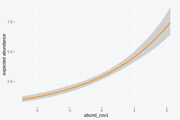
The curve climbs because the abundance slope is positive, and the
band carries the count uncertainty through the exponential. What lets
the model see eight animals through counts that never reach eight is the
spread of the counts across visits. A site that averages two animals per
visit could hold twenty seen one time in ten or three seen two times in
three, and the two readings produce counts with very different variance:
many animals at low detection jump around relative to their mean, few at
high detection barely move. The N-mixture reads that spread and infers
the abundance behind it, which is why replicate visits are not optional
here. The model also leans on closure, that the same animals stay put
across the survey window, so a season long enough to let animals move
violates it and reads the movement as detection noise.
abun(mixture = "negbin") adds an overdispersion parameter
for counts with more spread than a Poisson allows, common when animals
cluster, and the same icar() / bym2() terms
that smooth occupancy smooth a count surface. The closure assumption,
the count ceiling
,
the negative-binomial state, and areal spatial counts are in
vignette("abundance").
Community models
ms_occu() fits many species at once, with
community-level hyperpriors tying the species coefficients together so a
rare species borrows the shape of the assemblage. y is a
sites-by-visits-by-species array and species names the
third dimension. The community mean is the fixed effect
coef() returns.
sm <- simulate_ms_occu(N = 120, J = 5, n.species = 8, seed = 3)
fm <- tobs(~ x, data = sm$data, family = ms_occu(), detection = ~ 1,
           y = sm$y, species = paste0("sp", 1:8), method = "laplace",
           control = list(verbose = FALSE))
coef(fm, arm = "psi")                                # community occupancy mean
#> (Intercept)           x
#>  -0.1803196   0.5286092
tobs_richness() turns the per-species occupancy
posteriors into a site-level species-richness estimate with uncertainty,
summing occupancy probabilities across species rather than counting
detections. Plotting richness against site, ordered, shows the spread
across the survey with its band.
rich <- tobs_richness(fm)
rich <- rich[order(rich$mean), ]
rich$site <- seq_len(nrow(rich))
ggplot(rich, aes(x = site, y = mean)) +
  geom_ribbon(aes(ymin = q2.5, ymax = q97.5), alpha = 0.25, fill = "steelblue") +
  geom_line(colour = "steelblue", linewidth = 1) +
  labs(x = "site (ordered by richness)", y = "expected richness") +
  transparent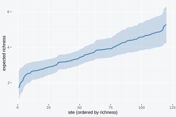
The modelled richness exceeds the naive detected count because it
adds the species probably present but undetected, and the band carries
every species’ occupancy uncertainty into the sum. The reason to fit the
assemblage jointly rather than species by species is the rare species. A
bird seen at three sites out of a hundred carries almost no information
on its own, and its single-species slope would run from deeply negative
to deeply positive. The community prior assumes the species coefficients
are draws from a shared distribution and pulls a thin species toward the
assemblage mean, hardest where its own data are weakest. The pull
strength is the fitted community covariance, learned from how the
species scatter rather than set by hand, so a homogeneous assemblage
pools hard and a heterogeneous one barely pools at all. The count
analogue is ms_abun(), the community N-mixture, which pools
abundance and detection across the assemblage the same way and exposes
per-species deviations through ranef(). When pooling helps,
when it hurts, and how to read the community covariance are in
vignette("community-models").
Cover hurdle
cover() fits a hurdle for continuous vegetation cover: a
binomial occurrence process on whether the species is present at all,
plus a positive-cover process (lognormal or beta) for how much ground it
covers where it occurs. The two arms fit as independent Laplace
approximations, and predict() reads occupancy and expected
cover at new covariate values.
sc <- simulate_cover(N = 400, beta.occ = c(-0.4, 0.7),
                     beta.pos = c(-1.0, 0.3), sigma.pos = 0.4, seed = 7)
fc <- tobs(~ x, data = sc$data, family = cover(response = "lognormal"),
           y = sc$y)
nd <- data.frame(x = seq(-2, 2, length.out = 50))
nd$expected <- predict(fc, nd, type = "expected")
head(nd)
#>           x   expected
#> 1 -2.000000 0.03160168
#> 2 -1.918367 0.03393849
#> 3 -1.836735 0.03643353
#> 4 -1.755102 0.03909579
#> 5 -1.673469 0.04193459
#> 6 -1.591837 0.04495957
The expected-cover curve combines both arms: the chance the species occurs times the cover it carries where it does. Plotting it across the covariate range traces the unconditional expected cover.
nd$occupancy <- predict(fc, nd, type = "occupancy")
ggplot(nd, aes(x = x, y = expected)) +
  geom_line(colour = "forestgreen", linewidth = 1) +
  labs(x = "x", y = "expected cover") +
  transparent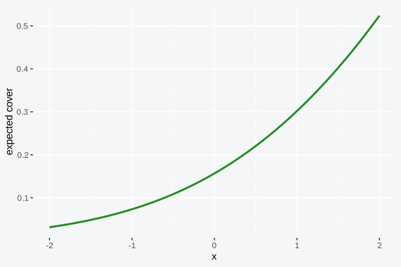
The rise reflects both a higher occurrence probability and more cover
where present as the covariate climbs. Cover data have a shape that
breaks an ordinary regression: a pile of exact zeros where the species
is absent, and a continuous positive distribution where it occurs.
Modelling the two together with one Gaussian forces a single mean to
explain both the zeros and the spread, and it predicts impossible
negative cover at the low end. The hurdle splits them, a binomial arm on
presence and a positive arm on the cover where present, so the zeros
inform occurrence and the positive values inform the cover distribution
without contaminating each other. The expected cover the plot shows is
the product of the two arms, which is why it can rise both because the
species occurs more often and because it covers more ground where it
does. This dispatcher predicts from fixed effects only; the shared-field
joint model, where occurrence, detection, and cover couple through one
spatial field, is the occu_cover() family. The
independent-arm hurdle is in vignette("cover-hurdle"), and
the joint engine in vignette("cover-hurdle-motivate").
Spatial occupancy
A neighbourhood graph lets adjacent regions share what the covariates
miss. An areal spatial field adds one smoothed random effect per cell,
ties neighbours together, and soaks up the part of occupancy that
depends on where a cell sits. The fields are formula terms:
icar(), bym2(), and car_proper(),
each taking a dense 0/1 adjacency matrix. They route through
method = "nested_laplace", which integrates the smoothing
strength over a grid.
gx <- 5; n <- gx * gx
coord <- expand.grid(cx = seq_len(gx), cy = seq_len(gx))
adj <- matrix(0, n, n)
for (i in seq_len(gx)) for (j in seq_len(gx)) {
  a <- (j - 1) * gx + i
  if (i < gx) { b <- (j - 1) * gx + i + 1; adj[a, b] <- adj[b, a] <- 1 }
  if (j < gx) { b <- j * gx + i;           adj[a, b] <- adj[b, a] <- 1 }
}
field <- 1.4 * exp(-((coord$cx - 3)^2 + (coord$cy - 3)^2) / 4)
field <- field - mean(field)
z <- rbinom(n, 1, plogis(field))
ys <- matrix(0L, n, 8L)
for (i in seq_len(n)) if (z[i]) ys[i, ] <- rbinom(8L, 1, 0.5)
fit_sp <- tobs(~ bym2(graph = adj), data = data.frame(site = seq_len(n)),
               family = occu(), detection = ~ 1, y = ys,
               method = "nested_laplace",
               control = list(max.iter = 30L, tol = 1e-5, verbose = FALSE))
predict(type = "state") returns the smoothed per-cell
occupancy posterior. Laying it back on the grid coordinates and shading
each cell maps the field, which peaks where the simulated bump put
it.
sp <- predict(fit_sp, type = "state")
mp <- cbind(coord, psi = sp$psi)
ggplot(mp, aes(x = cx, y = cy, fill = psi)) +
  geom_tile() +
  scale_fill_viridis_c() +
  labs(x = NULL, y = NULL, fill = "psi") +
  transparent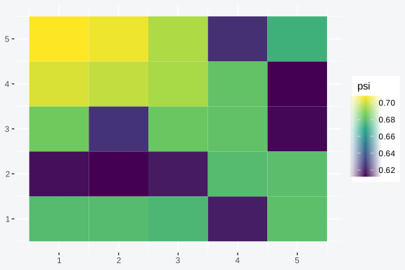
The high-occupancy ridge runs through the grid centre, smoothed from
the binary noise an isolated per-cell estimate would carry. The field
earns its keep two ways. It widens the slope standard errors to their
honest size, because adjacent cells share unmeasured drivers and a
non-spatial fit treats them as independent and runs its errors too
narrow. And it keeps a patterned covariate from absorbing the regional
signal it competes with, so the fitted slope reads against a background
that already accounts for location. The smoothing strength is itself a
parameter, and the nested path integrates it over a grid rather than
fixing it, so the slope errors inherit the field’s uncertainty instead
of pretending the smoothing was known. ICAR is the plain smoother, BYM2
splits structured from unstructured variation, and the proper CAR
estimates the autocorrelation strength. Areal fields, the floating
intercept under ICAR, and held-out-cell interpolation are in
vignette("spatial-occupancy"); continuous fields on point
coordinates are in vignette("occupancy-spatial-spde").
Dynamic occupancy
dyn_occu() fits the multi-season model of MacKenzie and
colleagues: a first-season occupancy, a colonisation rate for empty
sites, an extinction rate for occupied sites, and a detection process
over the latent state. The response carries a season dimension, and the
model sums the latent Markov chain out with the forward algorithm.
sd_dyn <- simulate_dyn_occu(N = 200, J = 4, n.seasons = 6,
                            beta.occ = c(0), beta.det = c(0),
                            gamma = 0.3, epsilon = 0.2, seed = 2026)
fit_dyn <- tobs(~ 1, data = sd_dyn$data, family = dyn_occu(),
                detection = ~ 1, y = sd_dyn$y,
                colonization = ~ 1, extinction = ~ 1,
                method = "laplace", control = list(verbose = FALSE))
fit_dyn$intercepts                          # psi1, p, gamma, epsilon
#> $psi1
#> psi1_(Intercept)
#>        0.4709663
#>
#> $p
#> p_(Intercept)
#>     0.5012209
#>
#> $gamma
#> gamma_(Intercept)
#>         0.2985127
#>
#> $epsilon
#> epsilon_(Intercept)
#>           0.2100606
The four rates land near their simulated values. The two transition rates imply an equilibrium occupancy , and iterating the transition forward from draws the modelled trajectory across seasons against the realised occupancy fractions.
g <- fit_dyn$intercepts$gamma; e <- fit_dyn$intercepts$epsilon
ns <- dim(sd_dyn$y)[3]; psi_t <- numeric(ns); psi_t[1] <- fit_dyn$intercepts$psi1
for (t in 2:ns) psi_t[t] <- psi_t[t - 1] * (1 - e) + (1 - psi_t[t - 1]) * g
tj <- data.frame(season = seq_len(ns), realised = colMeans(sd_dyn$truth$z),
                 modelled = psi_t)
ggplot(tj, aes(x = season)) +
  geom_line(aes(y = modelled), colour = "darkorange", linewidth = 1) +
  geom_point(aes(y = realised)) +
  ylim(0, 1) + labs(y = "occupied fraction") + transparent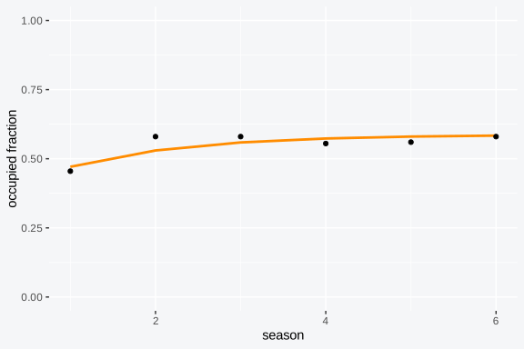
The modelled curve rises from the fitted starting occupancy toward
the equilibrium the rates imply, tracking the realised fractions. The
reason to estimate the two rates rather than occupancy alone is that the
same standing occupancy can come from opposite dynamics. A level holding
at sixty percent could be a placid system where the same sites stay
occupied for years, or a churning one where many sites wink out each
season and as many are colonised. The static occupancy is identical; the
rates tell them apart, and they imply different conservation responses.
The model reads the rates from the pattern of which sites change state
between consecutive seasons, which is why a multi-season survey is worth
the extra effort over repeating a single-season one. Covariates on
colonisation and extinction, turnover, and the count analogue
dyn_abun() are in
vignette("dynamic-occupancy").
Integrated occupancy
int_occu() combines several data sources that disagree
about detection but agree about occupancy. The sources share one latent
occupancy state and each carries its own detection process, so a
structured survey anchors the calibration while opportunistic records
extend the reach. y is a list of detection-history
matrices, one per source.
si <- simulate_int_occu(N.total = 500, n.data = 2, J = c(2, 5),
                        n.shared = 250, beta.occ = c(0.3, 0.9),
                        beta.det = list(c(0.5, 0), c(0.7, 0)), seed = 11)
fit_int <- tobs(~ x, data = si$data, family = int_occu(), detection = ~ 1,
                y = list(survey = si$y[[1]], casual = si$y[[2]]),
                method = "laplace", control = list(verbose = FALSE))
coef(fit_int, arm = "psi")                           # shared occupancy block
#> (Intercept)           x
#>   0.1627076   0.7712881
The fit returns one shared occupancy block plus a detection block per
source, keyed by the names you gave y. Plotting the two
detection intercepts on the probability scale shows each source’s
reporting rate, estimated separately.
dp <- data.frame(source = c("survey", "casual"),
                 p = plogis(c(coef(fit_int, arm = "survey"), coef(fit_int, arm = "casual"))))
ggplot(dp, aes(x = source, y = p)) +
  geom_col(fill = "steelblue", width = 0.5) +
  ylim(0, 1) + labs(x = NULL, y = "detection probability") +
  transparent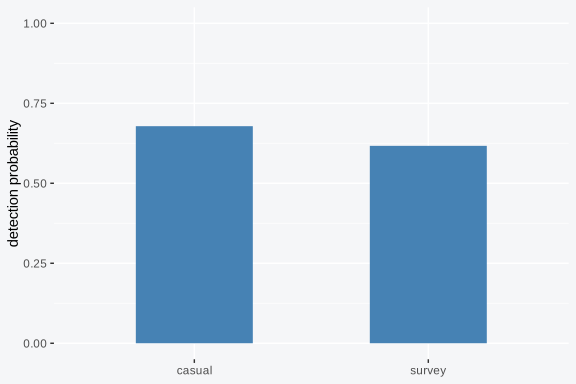
The two bars sit at different heights because the sources detect at
different rates, which is the point of the separate detection blocks.
The shared state borrows strength from both; the detection arms stay
independent. The logic that makes integration pay is that occupancy is a
property of the place and the species, not of who is looking, so a
structured survey and a casual stream can share one
while keeping their own
.
A single thin source has to estimate occupancy and its own detection
from a few visits, and the two trade off; a second source that observes
overlapping sites brings more visits to bear on the shared state without
forcing the detection processes to match. The gain scales with the
overlap and with how much real occupancy signal the added source
carries. Where integration sharpens the occupancy slope, the overlap
that drives the gain, and source-specific detection covariates are in
vignette("integrated-occupancy"). The joint species
distribution family jsdm() and the detection-protocol
families removal(), distance(), and
fp_occu() extend the same observation layer.
S3 methods
The fitted object answers the standard R accessors, and they behave
the same on a Laplace fit and a NUTS fit; the Laplace tier reports the
Gaussian approximation at the mode, the sampler tier reports empirical
posterior summaries. print() lays out both processes and
the family. summary() adds the standard deviation and
credible bounds, plus Rhat and effective sample size under
NUTS. coef() returns the estimates as a named vector,
confint() the credible intervals as a matrix, and
vcov() the fixed-effect covariance.
co  <- coef(fit)            # named <process>_<coefficient>
ci  <- confint(fit)         # matrix of credible bounds
vc  <- vcov(fit)            # fixed-effect covariance
list(coef = names(co), confint_rows = rownames(ci), vcov_dim = dim(vc))
#> $coef
#> [1] "psi_(Intercept)" "psi_occ_cov1"    "p_(Intercept)"   "p_det_cov1"
#>
#> $confint_rows
#> [1] "psi_(Intercept)" "psi_occ_cov1"    "p_(Intercept)"   "p_det_cov1"
#>
#> $vcov_dim
#> [1] 4 4
Beyond the four above, fitted() returns the per-site
psi, p, and z;
ranef() returns the group-level random effects when a model
carries them; residuals() returns deviance, Pearson, or
response residuals; predict() returns occupancy at a new
design or a varied term; and simulate() draws replicate
detection histories from the fit. The plot() method on a
prediction object draws the marginal-effect curve with its band, and on
a data object summarises the detection histories. The accessor surface
is deliberately the base-R one, so a tobs_fit drops into
code written for lm or glmer outputs.
The accessors that involve uncertainty read it from whichever
inference produced the fit, without you having to ask. On a Laplace fit,
confint() and vcov() come from the curvature
of the log-posterior at the mode, so they are the Gaussian approximation
and they return instantly. On a NUTS fit, the same calls summarise the
posterior draws, so the interval is the empirical quantile of the chain
and summary() carries the Rhat and
effective-sample-size columns alongside. The code you write does not
change between the two; only the numbers and their provenance do. That
is the practical payoff of keeping the observation layer thin and the
inference in the engine: you choose the backend per run and read the
result through one set of methods.
| Accessor | Returns |
|---|---|
coef() |
per-process fixed-effect estimates |
summary() |
estimate, SD, credible bounds (plus Rhat/ESS under NUTS) |
confint() |
credible intervals (matrix) |
vcov() |
fixed-effect covariance |
ranef() |
group-level random effects (when present) |
fitted() |
per-site psi, p, z
|
predict() |
occupancy at a new design or varied term |
waic() |
WAIC, elpd, effective parameters |
residuals() |
deviance / Pearson / response residuals |
simulate() |
replicate detection histories from the fit |
Practical guidance
-
Start with
method = "laplace". It is deterministic and returns in well under a second on a few hundred sites. Use it for the first look and for WAIC comparison. Move tomethod = "nuts"when detection is low, visits are few, or you need the full posterior shape rather than a Gaussian approximation at the mode. -
Visits drive identifiability. Occupancy and
detection trade off against each other. With two or three visits and
detection below about 0.3, the two processes are weakly separated and
the Laplace mode can drift; NUTS or more visits resolve it. The identifiability discussion in
vignette("occupancy")works through where recovery fails. -
Detection covariates broadcast across visits when
the data frame has one row per site, as in
simulate_occu(). For covariates that change between visits (effort, observer, weather), pass a per-visit design; seevignette("data-formatting"). -
Read uncertainty, not just point estimates.
confint()and thesummary()quantile columns carry the credible bounds. A coefficient whose interval spans zero is not pulling its weight regardless of the point estimate. -
WAIC compares, it does not validate. A lower WAIC
says one model predicts the in-sample data better; it does not say the
model is calibrated. Pair it with a posterior-predictive check
(
ppc(), seevignette("diagnostics")).
Where to go next
Single-season occupancy end to end, with model comparison and identifiability:
vignette("occupancy").N-mixture abundance, negative binomial, and areal spatial counts:
vignette("abundance").Many species at once:
vignette("community-models").Colonisation and extinction across seasons:
vignette("dynamic-occupancy").Combining detection histories from several sources:
vignette("integrated-occupancy").The vegetation cover hurdle, independent and joint:
vignette("cover-hurdle")andvignette("cover-hurdle-motivate").Areal and continuous spatial fields:
vignette("spatial-occupancy")andvignette("occupancy-spatial-spde").Random effects with
lme4bar syntax:vignette("random-effects").Posterior-predictive checks, WAIC, and spatial residual diagnostics:
vignette("diagnostics"). ```