Cover hurdle (independent arms) • tulpaObs

Installation

install.packages("pak")
pak::pak("gcol33/tulpaObs")            # latest from GitHub
pak::pak("gcol33/tulpaObs@v0.1.1")     # a specific tagged release

Tagged releases are listed at https://github.com/gcol33/tulpaObs/releases.

pak resolves the dependency tree, pulling tulpa and tulpaMesh from the r-universe repository DESCRIPTION declares in Additional_repositories, at or above the Imports floor. A C++17 toolchain is needed (Rtools on Windows, Xcode CLI tools on macOS, r-base-dev on Linux); both tulpa and tulpaObs compile their backends on first install.

Introduction

Vegetation cover comes with a pile of zeros. A plot either holds a species or it does not, and where the species is present its cover lands somewhere in $(0, 1]$ . Two questions ride on one column of data: where does the species occur, and how much of it is there once it occurs. A single Gaussian or beta regression on cover answers neither cleanly, because the zeros pull the fit one way and the positive values pull it another. A hurdle model splits the column into an occurrence arm and a positive-cover arm and lets each answer its own question.

This vignette fits the simplest version of that model: the two arms treated as independent. cover() under method = "laplace" runs a binomial GLM on the occurrence indicator and a separate Gaussian (or beta) GLM on the positive subset, with no field shared between them. That is the right tool when a zero always means true absence and the two processes are not tied through a common spatial signal. When they are tied, the joint shared-field model in vignette("cover-hurdle-motivate") couples the arms through one BYM2 field and a fitted copy coefficient; this vignette is the baseline that joint fit is measured against. The worked example runs end to end on simulate_cover() data where the generating parameters are known, so every estimate can be checked against a truth.

The fit uses two independent Laplace approximations through tulpa:

a binomial GLM on the occurrence indicator $\mathbf{1}\{y_i > 0\}$ ;
a Gaussian GLM on $\log y_i$ for the sites where $y_i > 0$ .

The shared-field joint model – occurrence, detection, and cover arms coupled through one spatial field – is the occu_cover() family; vignette("cover-hurdle-motivate") builds it end to end, including the beta positive variant. A separate-fit comparison against INLA::inla() on simulated data lives in vignette("cover-hurdle-vs-inla").

The model

Write $y_i$ for the cover at site $i$ on the natural $[0, 1]$ scale, with $y_i = 0$ recording absence. The hurdle splits $y_i$ into an occurrence indicator $z_i = \mathbf{1}\{y_i > 0\}$ and, where $z_i = 1$ , a positive part. The two arms carry their own coefficient vectors and are fit without any shared term:

$z_i \sim \mathrm{Bernoulli}(p_i), \qquad \operatorname{logit} p_i = \mathbf{x}_i^\top \boldsymbol\beta^{\mathrm{occ}},$ $y_i \mid z_i = 1 \sim f\!\left(\eta_i^{\mathrm{pos}}, \theta\right), \qquad \eta_i^{\mathrm{pos}} = \mathbf{x}_i^\top \boldsymbol\beta^{\mathrm{pos}} .$

Here $\mathbf{x}_i$ is the design row from the formula, $\boldsymbol\beta^{\mathrm{occ}}$ and $\boldsymbol\beta^{\mathrm{pos}}$ are the per-arm fixed effects, $p_i$ is the occurrence probability, and $\eta_i^{\mathrm{pos}}$ is the positive-arm linear predictor. The positive family $f$ comes in two variants. Under cover("lognormal") the engine fits a Gaussian on $\log y_i$ , so $\log y_i \mid z_i = 1 \sim \mathrm{Normal}(\eta_i^{\mathrm{pos}}, \sigma_{\mathrm{pos}}^2)$ , and the expected cover given presence back-transforms as $E[y_i \mid z_i = 1] = \exp(\eta_i^{\mathrm{pos}} + \sigma_{\mathrm{pos}}^2 / 2)$ . Under cover("beta") the engine fits a logit-link beta directly on $y_i$ with precision $\phi$ , so $\mu_i = \operatorname{logis}(\eta_i^{\mathrm{pos}})$ is the conditional mean and $\theta = \phi$ is the dispersion. Either way the expected cover combines the two arms as $E[y_i] = p_i \cdot \mu_i$ .

The two arms share nothing in this model. The occurrence coefficients are estimated from all $N$ sites; the positive coefficients are estimated from the $n_{\mathrm{pos}}$ sites with $y_i > 0$ only. That independence is exactly what the joint occu_cover() engine relaxes by tying the arms through a copy coefficient. The dispersion symbol $\theta$ stands in for either $\sigma_{\mathrm{pos}}$ (lognormal) or $\phi$ (beta), and the choice between the two families is the main modelling decision the practical guidance returns to.

The two positive variants differ in where they put their probability mass and in how they treat the cover scale. The lognormal variant models $\log y_i$ as Gaussian, so it lives on the multiplicative scale: a one-unit change in $\eta^{\mathrm{pos}}$ multiplies cover by a constant factor regardless of the baseline level, and the variance of cover grows with its mean. That matches a species whose cover ranges over orders of magnitude, from a trace patch to near full ground coverage, which is the common vegetation case. The lognormal puts no hard ceiling at one, so the engine clips simulated and predicted cover to the $[0, 1]$ range after the back-transform; in practice the ceiling rarely binds because the positive mass sits well below one. The beta variant models $y_i$ directly on the natural $(0, 1)$ scale with a logit link on the mean and a single precision $\phi$ that controls the spread. Its variance $\mu(1 - \mu) / (1 + \phi)$ shrinks toward both boundaries, so it fits cover that clusters in the middle of the unit interval and respects the ceiling at one without clipping. The occurrence arm is identical under both, a plain binomial on the indicator, so swapping the positive family changes only how the above-zero values are described.

Simulating data

simulate_cover() generates data from exactly this generative model. It draws one continuous covariate x, builds both linear predictors from the supplied coefficient vectors, draws the occurrence indicator from a Bernoulli, and draws log-cover from a Gaussian on the occupied sites before exponentiating back to the natural scale. The covariate enters both arms with its own slope, so the simulator can produce a species whose occurrence rises with x while its conditional cover falls, which is the case the hurdle split is built to separate.

library(tulpaObs)
sim <- simulate_cover(
  N         = 400,
  beta.occ  = c(-0.4, 0.7),
  beta.pos  = c(-1.0, 0.3),
  sigma.pos = 0.4,
  seed      = 7
)
head(sim$data)
#>       cover          x       lon       lat
#> 1 1.0000000  2.2872472 0.3745957 0.1097551
#> 2 0.1891462 -1.1967717 0.4804525 0.8830442
#> 3 0.0000000 -0.6942925 0.8780038 0.5533614
#> 4 0.0000000 -0.4122930 0.7827960 0.4722463
#> 5 0.0000000 -0.9706733 0.2670661 0.3544873
#> 6 0.0000000 -0.9472799 0.1044755 0.9312948

The returned sim$data carries the cover values, the covariate x, and a pair of coordinates lon / lat that the non-spatial fit ignores. The cover vector itself is sim$y, the object passed to tobs() through the y argument. The generating parameters sit in sim$truth: the occurrence coefficients beta_occ, the positive-cover coefficients beta_pos, the lognormal residual SD sigma_pos, plus the per-site occurrence probability p, the conditional mean cover mu, and the realized occurrence indicator occur.

c(
  n_sites    = length(sim$y),
  n_positive = sum(sim$y > 0),
  prevalence = mean(sim$y > 0),
  median_pos = median(sim$y[sim$y > 0])
)
#>     n_sites  n_positive  prevalence  median_pos 
#> 400.0000000 171.0000000   0.4275000   0.3990295

Prevalence near one half on 400 sites leaves roughly 200 positive observations for the cover arm, comfortably above the coefficient count. The two arms see different sample sizes by construction: every site informs occurrence, only the occupied ones inform cover. A picture of the response makes the zero spike and the right-skewed positive tail visible, which is the structure that motivates the hurdle in the first place.

library(ggplot2)
df <- data.frame(cover = sim$y, occupied = sim$y > 0)
ggplot(df, aes(cover, fill = occupied)) +
  geom_histogram(bins = 40, colour = NA) +
  labs(x = "cover", y = "count", fill = "y > 0") +
  theme(panel.background = element_rect(fill = "transparent"),
        plot.background  = element_rect(fill = "transparent"))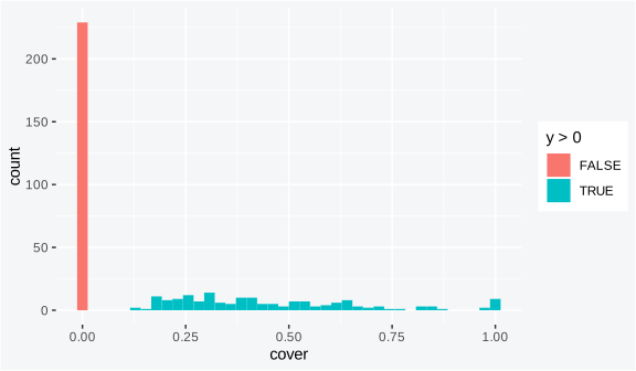

The tall bar at zero is the absence spike; the spread of positive values is the cover-arm signal. A Gaussian fit on the whole column would try to straddle both and land badly between them. The hurdle fits the spike with a binomial and the spread with the positive family, each on its own data.

The simulator exposes the knobs that matter for the fit’s behaviour. beta.occ sets the occurrence intercept and slope, so lowering the intercept thins the positives and raising the slope sharpens the dependence of presence on x; beta.pos does the same for conditional cover. sigma.pos is the lognormal residual SD, the width of the positive distribution on the log scale, and shrinking it tightens the cover values around the fitted curve. The seed argument fixes the random draw so the example reproduces exactly, which is what lets the recovery table below compare estimates to the named truth rather than to a moving target. Changing N trades sampling noise for compute: more sites narrow every interval, and the recovery tolerances in the package’s own tests loosen visibly as N drops from 800 toward 200. For a first look at a real dataset, simulating from coefficients in the rough neighbourhood of the data’s prevalence and median cover is a quick way to see how tight the intervals will be before fitting the real thing.

Fitting

The fit is one tobs() call. The formula carries the fixed effects shared by both arms (here a single covariate x), the data frame supplies the design, the family is cover(response = "lognormal"), and the cover values pass through y. The default method = "auto" resolves to "laplace" for the cover family, which is the two-independent-Laplace path; nothing else needs setting for the non-spatial fit.

fit <- tobs(
  formula = ~ x,
  data    = sim$data,
  family  = cover(response = "lognormal"),
  y       = sim$y
)
fit
#> <cover_fit (lognormal positive part)>
#>   N total      : 400
#>   N positive   : 171 (42.8%)
#>   sigma_pos    : 0.3838
#>   converged    : yes
#> 
#> Presence (binomial logit):
#>               estimate   std.err   z.value
#> (Intercept) -0.3514232 0.1069681 -3.285309
#> x            0.6583625 0.1150473  5.722539
#> 
#> Positive (Gaussian on log y > 0):
#>               estimate    std.err   z.value
#> (Intercept) -1.0424600 0.03155631 -33.03492
#> x            0.3223995 0.02945743  10.94459

The print method lays out both arms. The header reports the positive family, the total and positive sample sizes, the fitted residual SD sigma_pos, and the convergence flag. The occurrence block is the binomial-logit fit on $z_i$ ; the log-cover block is the Gaussian fit on $\log y_i$ over the positive subset. Each block shows the coefficient estimate and its standard error per term, so the slope on x can be read off directly for each process.

The fitted object is a cover_fit, and the two arms are reachable as named vectors. beta_occ and se_occ are the occurrence coefficients and their SEs; beta_pos and se_pos are the positive-arm coefficients and SEs. The lognormal residual SD is sigma_pos (a scalar). Pulling them into a table puts the estimates next to the generating truth.

est <- data.frame(
  parameter = c("beta_occ_(Intercept)", "beta_occ_x",
                "beta_pos_(Intercept)", "beta_pos_x", "sigma_pos"),
  truth     = c(sim$truth$beta_occ, sim$truth$beta_pos, sim$truth$sigma_pos),
  estimate  = c(fit$beta_occ, fit$beta_pos, fit$sigma_pos),
  se        = c(fit$se_occ, fit$se_pos, NA)
)
print(est, row.names = FALSE, digits = 3)
#>             parameter truth estimate     se
#>  beta_occ_(Intercept)  -0.4   -0.351 0.1070
#>            beta_occ_x   0.7    0.658 0.1150
#>  beta_pos_(Intercept)  -1.0   -1.042 0.0316
#>            beta_pos_x   0.3    0.322 0.0295
#>             sigma_pos   0.4    0.384     NA

The occurrence slope recovers near its generating value of +0.7 and the positive-cover slope near +0.3, each within a couple of SEs. The residual SD sigma_pos lands near the generating 0.4. One detail to keep in mind: tulpa::tulpa_laplace(family = "gaussian") runs with the dispersion fixed at one and the cover arm estimates sigma_pos post-hoc as the residual standard error $\sqrt{\mathrm{SS}_{\mathrm{res}} / (n_{\mathrm{pos}} - p)}$ . That is why sigma_pos has no SE column here, and why its intercept partner beta_pos absorbs whatever residual scale the engine attributes to the data. The occurrence arm carries no dispersion parameter at all, being a binomial with the trial count fixed at one.

Two arms means two convergence states folded into one flag. converged(fit) is TRUE only when both the binomial and the Gaussian Laplace solves converged, so a single number reports the health of the whole hurdle. The per-arm marginal likelihoods sit in fit$log_marginal under the names occ and pos, which the model-comparison section uses.

The fit also stamps the design it actually used onto fit$encoding, which is worth knowing for two reasons. First, the engine autoscales the numeric columns of each arm’s design matrix so the optimizer sees well-conditioned predictors, then transforms the coefficients and SEs back to the natural scale before returning them, so the beta_occ and beta_pos you read are on the same scale as the covariate, not the scaled one. Second, the encoding records which rows fell into the positive subset and how many positive observations each arm saw, which the convergence flag and the too-few-positives guard both lean on. If the positive subset has fewer than ncol(X) + 1 rows the fit stops with an error rather than returning an unidentified cover arm, because a Gaussian on fewer points than coefficients has no residual degrees of freedom to estimate sigma_pos from. Swapping the family to cover("beta") keeps the same call and the same extraction, with phi_pos replacing sigma_pos as the dispersion and the positive block printing as a logit-link beta.

Checking the fit

A fit that printed cleanly can still be wrong, so the two arms get checked separately against the data they were fit on. The occurrence arm is a binomial, so the natural check is calibration: bin sites by their predicted occupancy probability and compare the predicted rate in each bin to the observed occurrence rate. If the binomial link and linear predictor are right, the two track the diagonal.

p_hat <- predict(fit, sim$data, type = "occupancy")
bins  <- cut(p_hat, breaks = seq(0, 1, by = 0.1), include.lowest = TRUE)
cal   <- aggregate(list(observed = as.integer(sim$y > 0)),
                   by = list(bin = bins), FUN = mean)
cal$predicted <- tapply(p_hat, bins, mean)[cal$bin]

ggplot(cal, aes(predicted, observed)) +
  geom_abline(linetype = 2) +
  geom_point(size = 2) +
  labs(x = "predicted occupancy", y = "observed occurrence rate") +
  theme(panel.background = element_rect(fill = "transparent"),
        plot.background  = element_rect(fill = "transparent"))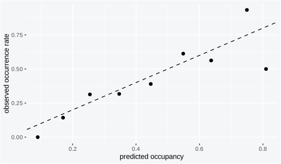

The points fall close to the dashed diagonal across the probability range, which is what a well-calibrated occurrence arm looks like. Departures would show up as points sitting systematically above or below the line in a region of predicted probability, signalling a missing covariate or a link mismatch. A single numeric summary of the same idea is the agreement between mean predicted occupancy and overall prevalence.

c(mean_predicted = mean(p_hat), observed_prevalence = mean(sim$y > 0))
#>      mean_predicted observed_prevalence 
#>           0.4275001           0.4275000

The positive arm is a Gaussian on $\log y_i$ , so its check is a residual look on the log scale. Standardized residuals against the fitted log-cover should sit in a flat band around zero with no funnel and no trend; a funnel would mean the constant-variance assumption is off, and a trend would mean a missing covariate on the cover arm.

pos       <- sim$y > 0
eta_pos   <- as.numeric(model.matrix(~ x, sim$data)[pos, ] %*% fit$beta_pos)
resid_std <- (log(sim$y[pos]) - eta_pos) / fit$sigma_pos

ggplot(data.frame(fitted = eta_pos, resid = resid_std), aes(fitted, resid)) +
  geom_hline(yintercept = 0, linetype = 2) +
  geom_point(alpha = 0.4) +
  labs(x = "fitted log-cover", y = "standardized residual") +
  theme(panel.background = element_rect(fill = "transparent"),
        plot.background  = element_rect(fill = "transparent"))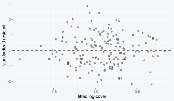

The residuals scatter evenly around zero with no fanning, so the lognormal arm’s constant-variance assumption holds on this data, as it should given the simulator drew log-cover with a fixed sigma_pos. On real data a visible funnel would argue for the beta family instead, whose variance shrinks toward the $(0, 1)$ boundaries. The standardized residuals should also look roughly standard-normal, which a quick spread check confirms.

c(resid_sd = sd(resid_std), frac_within_2 = mean(abs(resid_std) < 2))
#>      resid_sd frac_within_2 
#>     0.9970545     0.9590643

A standard deviation near one and about 95% of residuals inside $\pm 2$ are the marks of a Gaussian arm fitting its data. These checks are deliberately built from the fit’s own coefficients and predict() rather than from the single-season occupancy diagnostics (ppc(), pit_residuals()), which operate on replicated detection data and do not apply to the plot-level cover hurdle.

The two checks divide cleanly because the arms are independent here. The calibration plot exercises the occurrence arm alone, since it compares predicted occupancy to observed presence and never touches the cover values. The residual plot exercises the positive arm alone, since it runs over the occupied sites and never touches the zeros. Nothing couples them in this model, so a failure in one plot localizes to one arm and one set of coefficients, which is faster to act on than a single joint diagnostic that mixes both. On a real dataset the most common finding is a calibration plot that bows away from the diagonal at high predicted occupancy, which points to a saturating covariate or a missing interaction on the occurrence formula, and a residual funnel on the positive arm that argues for the beta family. Both are fixes to the formula or the family rather than to the engine, and re-running the same two chunks after the change confirms whether the fix landed.

Interpreting results

The coefficients are posterior summaries, so each comes with a credible interval rather than a bare point. With a Laplace fit the interval is the Wald band $\hat\beta \pm 1.96\,\mathrm{SE}$ on each arm, read straight off beta_occ / se_occ and beta_pos / se_pos. The occurrence slope is the change in occurrence logit per unit x; the positive slope is the change in conditional log-cover per unit x.

z   <- qnorm(0.975)
ci  <- data.frame(
  parameter = c("beta_occ_(Intercept)", "beta_occ_x",
                "beta_pos_(Intercept)", "beta_pos_x"),
  estimate  = c(fit$beta_occ, fit$beta_pos),
  lwr       = c(fit$beta_occ, fit$beta_pos) - z * c(fit$se_occ, fit$se_pos),
  upr       = c(fit$beta_occ, fit$beta_pos) + z * c(fit$se_occ, fit$se_pos)
)
print(ci, row.names = FALSE, digits = 3)
#>             parameter estimate    lwr    upr
#>  beta_occ_(Intercept)   -0.351 -0.561 -0.142
#>            beta_occ_x    0.658  0.433  0.884
#>  beta_pos_(Intercept)   -1.042 -1.104 -0.981
#>            beta_pos_x    0.322  0.265  0.380

Both slopes on x have intervals clear of zero, so the covariate moves both occurrence and conditional cover credibly. The two effects are on different scales (logit on the occurrence arm, log-cover on the positive arm), so the more readable summary is the expected cover across the covariate range, with a band. Expected cover is $E[y] = p \cdot \mu$ , and propagating the per-arm SEs through that product gives an approximate band. The cleanest route is to draw coefficients from each arm’s Gaussian posterior, push every draw through the prediction, and take per-x quantiles, which carries the curvature of the logit and lognormal links rather than a linearization.

newdata <- data.frame(x = seq(-2, 2, length.out = 60))
Xn      <- model.matrix(~ x, newdata)
S       <- 2000L
draw    <- function(m, se) sweep(matrix(rnorm(S * length(m)), S), 2, se, "*") +
                           rep(m, each = S)
B_occ   <- draw(fit$beta_occ, fit$se_occ)
B_pos   <- draw(fit$beta_pos, fit$se_pos)
E_draws <- plogis(B_occ %*% t(Xn)) * exp(B_pos %*% t(Xn) + fit$sigma_pos^2 / 2)
band    <- data.frame(x = newdata$x, mean = colMeans(E_draws),
                      lwr = apply(E_draws, 2, quantile, 0.025),
                      upr = apply(E_draws, 2, quantile, 0.975))

Each draw is a coefficient pair sampled from the per-arm Gaussian posterior, pushed through the full prediction, so the band carries the link curvature rather than a delta-method linearization.

ggplot(band, aes(x, mean)) +
  geom_ribbon(aes(ymin = lwr, ymax = upr), alpha = 0.2) +
  geom_line() +
  labs(x = "x", y = "expected cover E[y]") +
  theme(panel.background = element_rect(fill = "transparent"),
        plot.background  = element_rect(fill = "transparent"))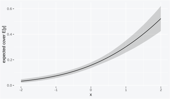

The curve rises with x because the occurrence slope dominates the product, and the band widens at the extremes where the covariate has fewer supporting sites. Reading the curve without the band would overstate confidence in the tails. The band here treats the two arms as independent, which they are in this model, so the interval is the per-arm uncertainty combined through the product and no cross-arm covariance is folded in.

Prediction

predict() on a cover_fit returns one of three quantities at new covariate values, selected by type. type = "occupancy" returns the occurrence probability $p = \operatorname{logis}(\mathbf{x}^\top \boldsymbol\beta^{\mathrm{occ}})$ ; type = "conditional" returns the conditional mean cover $\mu$ (the lognormal back-transform $\exp(\eta^{\mathrm{pos}} + \sigma_{\mathrm{pos}}^2 / 2)$ , or $\operatorname{logis}(\eta^{\mathrm{pos}})$ under beta); and type = "expected" returns their product $E[y] = p \cdot \mu$ . The three are linked by an exact identity, expected equals occupancy times conditional, which holds row by row.

newdata <- data.frame(x = seq(-2, 2, length.out = 50))
preds <- data.frame(
  x         = newdata$x,
  occupancy = predict(fit, newdata, type = "occupancy"),
  expected  = predict(fit, newdata, type = "expected")
)
head(preds)
#>           x occupancy   expected
#> 1 -2.000000 0.1586712 0.03160168
#> 2 -1.918367 0.1659780 0.03393849
#> 3 -1.836735 0.1735519 0.03643353
#> 4 -1.755102 0.1813962 0.03909579
#> 5 -1.673469 0.1895138 0.04193459
#> 6 -1.591837 0.1979068 0.04495957

The newdata frame needs the same covariate columns the formula used; a mismatch on column count or name errors rather than guessing. The prediction is fixed-effects only, which is all this dispatcher carries: there is no spatial field to project at new locations in the independent-arm path. A plot of all three curves at once shows how the expected cover is the occupancy curve scaled down by the conditional-cover curve.

qty   <- c("occupancy", "conditional", "expected")
long3 <- do.call(rbind, lapply(qty, function(q) data.frame(
  x = newdata$x, quantity = q, value = predict(fit, newdata, type = q))))

Stacking the three prediction types into long form lets one ggplot() layer all three curves with a shared colour scale, which makes the occupancy-times- conditional structure of expected cover read at a glance.

ggplot(long3, aes(x, value, colour = quantity)) +
  geom_line(linewidth = 0.8) +
  labs(x = "x", y = "prediction", colour = NULL) +
  theme(panel.background = element_rect(fill = "transparent"),
        plot.background  = element_rect(fill = "transparent"))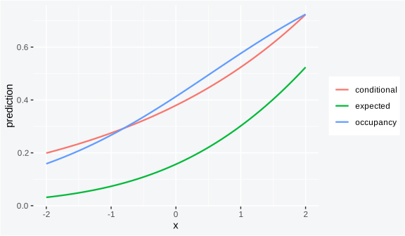

The occupancy curve climbs toward one as x rises, the conditional cover drifts up gently with its smaller slope, and the expected cover tracks their product. At low x the expected cover is pulled down by the low occupancy even where conditional cover is moderate, which is the hurdle structure showing through: near-zero expected cover comes from near-zero occurrence, not from low cover where the species is present. Confirming the identity numerically is a one-line check.

e <- predict(fit, newdata, type = "expected")
pm <- predict(fit, newdata, type = "occupancy") *
      predict(fit, newdata, type = "conditional")
max(abs(e - pm))
#> [1] 0

The maximum gap is at numerical-tolerance level, confirming that type = "expected" is exactly the product of the other two and not a separately fit surface.

Which prediction type to report depends on the question. Occupancy answers where the species is likely to occur and is the right map for a presence survey or a range estimate. Conditional cover answers how dense the species is where it does occur and is the right quantity for a biomass or competition argument, but it is silent about the zeros and so overstates the average cover across a landscape that includes empty plots. Expected cover folds the two together and is the honest landscape average, the quantity a monitoring programme usually wants, because a plot contributes its conditional cover weighted by how likely the species is to be there at all. The three predictions are fixed-effects only in this dispatcher, so they extrapolate the fitted covariate relationship to the newdata covariate values without any spatial adjustment; a site far outside the covariate range seen in training gets a prediction driven entirely by the extrapolated linear predictor, which the widening band in the interpretation plot already flagged. For the spatial case, where a fitted field would shift the prediction at a known location, the joint occu_cover() engine carries the projection machinery this dispatcher does not.

Model comparison

The positive family is a modelling choice, and the hurdle is fully observed, so WAIC is available to score it. waic() assembles the pointwise log-likelihood across both arms (the occurrence Bernoulli plus, where $y_i > 0$ , the positive-part density) and returns the WAIC, the expected log-pointwise predictive density elpd, the effective number of parameters p_waic, and the log-pointwise predictive density lppd. Fitting the same data with the lognormal and beta positive arms and scoring both is the cleanest way to decide which positive family the data prefers.

fit_ln   <- tobs(~ x, data = sim$data, family = cover("lognormal"), y = sim$y)
fit_beta <- tobs(~ x, data = sim$data, family = cover("beta"),      y = sim$y)

waic_ln   <- waic(fit_ln)
waic_beta <- waic(fit_beta)

The two fits share the occurrence arm exactly (the Bernoulli sees the same zeros), so the WAIC difference is driven entirely by how well each positive family describes the spread of cover above zero. A lower WAIC is the better fit on this scoring.

comparison <- data.frame(
  positive = c("lognormal", "beta"),
  waic     = c(waic_ln$estimates["waic", "Estimate"], waic_beta$estimates["waic", "Estimate"]),
  elpd     = c(waic_ln$estimates["elpd_waic", "Estimate"], waic_beta$estimates["elpd_waic", "Estimate"]),
  p_waic   = c(waic_ln$estimates["p_waic", "Estimate"], waic_beta$estimates["p_waic", "Estimate"])
)
comparison$delta_waic <- comparison$waic - min(comparison$waic)
print(comparison, row.names = FALSE, digits = 4)
#>   positive  waic   elpd p_waic delta_waic
#>  lognormal 359.2 -179.6  3.800       0.00
#>       beta 424.7 -212.3  6.646      65.48

Because this data was simulated from the lognormal generative model, the lognormal arm should score at or below the beta arm here, and a delta_waic larger than a few units on the wrong family is the signal to switch. On real cover data the verdict can go either way: cover concentrated in the middle of $(0, 1)$ favours beta, while cover with many small-but-positive values and a long right tail favours lognormal. The WAIC difference is the number to report, but it should be read alongside the conditional-cover residual check above, because WAIC rewards the family that fits the bulk of the data and can miss a boundary misfit that the residual plot makes obvious.

The same waic() call also scores the hurdle against a simpler nested model, for instance an intercept-only cover formula versus the covariate model, which tests whether x earns its place on the arms. The comparison is valid as long as both fits are scored on the same response with the same WAIC assembly, which waic() guarantees by reading each fit’s own encoding.

Practical guidance

A few numbers and rules of thumb that hold up across the recovery tests.

At least ncol(X) + 1 positive observations, and comfortably more. The positive arm only sees the sites with $y_i > 0$ . The encoder hard-errors below ncol(X) + 1 positive rows, but that floor is a structural minimum, not a working target. Aim for roughly 20 to 30 positive observations per cover-arm coefficient; a two-covariate cover formula wants the positive subset well into the dozens before the slopes and sigma_pos settle. The recovery tests run at 600 to 800 sites with prevalence near one half, which leaves a few hundred positive rows, and even there the per-fit sigma_pos carries a tolerance of about 15% around its truth.
Prevalence away from the extremes. With prevalence below roughly 0.1 the occurrence arm has few positives to estimate the slope from and the cover arm has few observations at all; with prevalence above 0.95 the occurrence arm has few zeros and the binomial slope is poorly pinned. The simulator’s default coefficients keep prevalence in a workable middle band, and a real dataset with prevalence at an extreme should expect wide intervals on the corresponding arm.
Sample size scales the sigma_pos agreement. The lognormal residual SD is computed post-hoc and converges to the generating value as the positive subset grows. At a few hundred positive rows it lands within about 15% of truth; at a few dozen it can be off by more, which then feeds through the lognormal back-transform and scales every conditional-cover prediction. When the positive subset is small, treat sigma_pos and the conditional-cover curve as the least certain outputs of the fit.

Choosing the positive family comes down to where the cover mass sits. Use cover("lognormal") when cover is right-skewed with many small-but-positive values and a long upper tail, which is the common vegetation pattern; the Gaussian-on-log fit handles the skew and the residual check on the log scale is easy to read. Use cover("beta") when cover is bounded strictly inside $(0, 1)$ and concentrated in the middle, where the beta’s shrinking variance toward the boundaries matches the data and the lognormal would overstate the spread near one. When the call is genuinely close, fit both and compare WAIC as above, then confirm the winner with the conditional-cover residual plot, because the two diagnostics catch different failures.

When to use the joint occu_cover() instead: the independent-arm cover() model here assumes the two arms share no structure and that a zero always means true absence. Reach for the joint shared-field model in vignette("cover-hurdle-motivate") when either assumption fails. If a habitat gradient that lifts occurrence also lifts conditional cover, the arms are coupled through a common spatial field and fitting them apart throws that coupling away along with the cover observations’ information about occurrence at neighbouring plots; the joint fit recovers a copy coefficient alpha with a credible interval that formally tests whether the coupling is real. And if a zero can mean the species was present but missed, the three-arm occu_cover() adds a detection layer that separates non-detection from absence, which the plot-level cover() cannot do because it has no replicated visits. With fewer than roughly 30 spatial units the shared field is weakly identified and the joint machinery buys little, so the independent-arm fit here, with spatial structure folded into covariates, is the more honest model at small N. The joint path stays affordable on large resurvey datasets because it collapses both arms to exact sufficient statistics before each inner solve (control$aggregate.occ and control$aggregate.pos, both on by default and byte-identical to the full per-plot fit); vignette("cover-hurdle-motivate") shows those controls.

# The equivalent joint hurdle in INLA, for comparison on the MOTIVATE
# resurvey data.
#
# library(INLA)
# joint <- inla(
#   list(
#     occur ~ x + f(site, model = "bym2", graph = adj),
#     log_cover ~ x + f(site, model = "bym2", graph = adj, copy = "site",
#                       fixed = FALSE)
#   ),
#   family = c("binomial", "gaussian"),
#   data   = inla_stack
# )

Scope

This dispatcher predicts from fixed effects only. Spatial fields fit through the spatial argument, and spatial projection at new coordinates – together with the within/between (Mundlak) temporal decomposition – comes with the joint occu_cover() engine; see vignette("cover-hurdle-motivate").