Installation
install.packages("pak")
pak::pak("gcol33/tulpaObs")            # latest from GitHub
pak::pak("gcol33/tulpaObs@v0.1.1")     # a specific tagged release
Tagged releases are listed at https://github.com/gcol33/tulpaObs/releases.
pak resolves the dependency tree, pulling tulpa and
tulpaMesh from the r-universe repository DESCRIPTION
declares in Additional_repositories, at or above the
Imports floor. A C++17 toolchain is needed (Rtools on
Windows, Xcode CLI tools on macOS, r-base-dev on Linux);
both tulpa and tulpaObs compile their backends
on first install.
Two pieces: the response and the site table
Every tobs() call takes a detection response
y and a per-site data frame. The formula on
the left of the call names columns in data; the
detection formula names columns there too. The shape of
y is what changes between families, and getting it right is
most of the work.
For single-season occupancy, y is an N x J
matrix: one row per site, one column per visit, holding 0
(surveyed, not detected), 1 (detected), or NA
(not surveyed). The data frame has exactly N
rows, one per site, aligned to the rows of y. A small
simulated dataset shows the layout.
sim <- simulate_occu(
  N = 120, J = 5,
  n.occ.covs = 1, n.det.covs = 1,
  beta.occ = c(0.2, 0.9),
  beta.det = c(0.5, 0.4),
  seed = 1
)
y   <- sim$y
dat <- sim$data
dim(y)
#> [1] 120   5
y[1:4, ]
#>      [,1] [,2] [,3] [,4] [,5]
#> [1,]    0    0    1    0    0
#> [2,]    0    1    1    0    1
#> [3,]    0    1    1    1    0
#> [4,]    0    0    0    0    0
head(dat, 4)
#>     occ_cov1   det_cov1
#> 1 -0.6264538 -0.5059575
#> 2  0.1836433  1.3430388
#> 3 -0.8356286 -0.2145794
#> 4  1.5952808 -0.1795565
The matrix has 120 rows to match the 120 rows in dat.
Row i of y is the detection history for the
site described by row i of dat. That alignment
is the contract tobs() checks first, and it is the one to
get right before anything else.
The other families reshape the same idea:
| Family |
y shape |
|---|---|
| Single-season occupancy, N-mixture |
N x J matrix |
Community (ms_occu, ms_abun) |
N x J x species array |
Dynamic (dyn_occu) |
N x J x season array |
Integrated (int_occu) |
list of matrices, one per source |
In every case the leading dimension is the site, the second is the
visit, and data carries one row per site.
Site-level versus visit-level covariates
Occupancy covariates describe a site and do not change between
visits, so they live as plain columns in data. Detection
covariates can vary by visit (effort, observer, weather). When
data has one row per site, a detection covariate named in
the detection formula is read from that single row and
broadcast across all J visits. That is the common case, and
it is what the simulators produce.
fit <- tobs(
  ~ occ_cov1,
  data      = dat,
  family    = occu(),
  detection = ~ det_cov1,
  y         = y,
  method    = "laplace",
  control   = list(verbose = FALSE)
)
coef(fit)
#> psi_(Intercept)    psi_occ_cov1   p_(Intercept)      p_det_cov1
#>       0.3625745       0.9012885       0.3668280       0.5797823
occ_cov1 and det_cov1 both came out of
dat. The occupancy slope used the value once per site; the
detection slope used the same value for each of the five visits at that
site. When a detection covariate genuinely changes between visits you
supply a per-visit design instead of a single site value, which the
tobs_data() helper below builds for you from a long
table.
Building y from a long detection table
Field data rarely arrives as a wide matrix. The usual starting point
is a long table with one row per site-visit: a site id, a visit number,
and a 0/1 detection. Reshaping that into the N x J matrix
is a reshape() or a matrix-indexing step.
long <- data.frame(
  site     = rep(paste0("S", 1:6), each = 3),
  visit    = rep(1:3, times = 6),
  detected = rbinom(18, 1, 0.4),
  elev     = rep(rnorm(6), each = 3)   # a site-level covariate
)
head(long, 6)
#>   site visit detected       elev
#> 1   S1     1        0  0.8816725
#> 2   S1     2        0  0.8816725
#> 3   S1     3        0  0.8816725
#> 4   S2     1        0 -0.9745003
#> 5   S2     2        0 -0.9745003
#> 6   S2     3        0 -0.9745003
The direct route fills a matrix by indexing on the site and visit
positions. Build the empty matrix at the right size, then scatter each
row of the long table into its [site, visit] cell.
sites  <- sort(unique(long$site))
visits <- sort(unique(long$visit))
ymat   <- matrix(NA_integer_, length(sites), length(visits),
                 dimnames = list(sites, paste0("V", visits)))
si <- match(long$site,  sites)
vi <- match(long$visit, visits)
ymat[cbind(si, vi)] <- as.integer(long$detected)
ymat
#>    V1 V2 V3
#> S1  0  0  0
#> S2  0  0  0
#> S3  0  0  0
#> S4  0  1  0
#> S5  0  0  1
#> S6  1  0  1
The site-level table then takes one row per site, in the same site order as the matrix rows.
site_dat <- long[match(sites, long$site), "elev", drop = FALSE]
rownames(site_dat) <- NULL
site_dat
#>          elev
#> 1  0.88167254
#> 2 -0.97450027
#> 3  0.39910492
#> 4 -0.41543326
#> 5 -0.01865714
#> 6  1.57122440
tobs_data() packages both steps. Hand it the long frame
and the column names; it returns a tobs_data object
carrying the detection matrix, the site-level covariates, and any
visit-level detection covariates as their own N x J
matrices.
obs <- tobs_data(
  long,
  y     = "detected",
  site  = "site",
  visit = "visit",
  occ.covs = "elev"
)
obs
#> tobs_data: 6 sites, 3 visits
#>   Occupancy covariates: elev
str(obs$y)
#>  int [1:6, 1:3] 0 0 0 0 0 1 0 0 0 1 ...
#>  - attr(*, "dimnames")=List of 2
#>   ..$ : chr [1:6] "S1" "S2" "S3" "S4" ...
#>   ..$ : NULL
obs$y is the same 6 x 3 matrix, with site
ids on the rows. obs$occ.covs holds the per-site
elev column. A detection covariate passed through
det.covs would come back as its own N x J
matrix rather than a single column, so a per-visit value lands in the
right visit slot.
The type argument controls what the response column
means. The default, "occurrence", builds an integer 0/1
matrix; "abundance" keeps integer counts;
"cover" keeps a continuous proportion in
[0, 1] without coercing it to integer. Picking the wrong
one is a common quiet error: a cover value of 0.6 run
through the integer path truncates to 0. The same long
frame can feed an occurrence and a cover model side by side as long as
each call names the matching column and type.
cov_long <- data.frame(
  site  = rep(paste0("S", 1:4), each = 2),
  visit = rep(1:2, times = 4),
  cover = round(runif(8, 0, 0.8), 2)
)
cov_obs <- tobs_data(cov_long, y = "cover", site = "site", visit = "visit",
                     type = "cover")
cov_obs$y
#>    [,1] [,2]
#> S1 0.45 0.68
#> S2 0.73 0.21
#> S3 0.31 0.35
#> S4 0.50 0.23
Building a tobs_data object by hand
When the matrix and covariates already sit in the right shape, skip
the long frame and assemble the object directly.
tobs_format() is the low-level constructor: it wraps a
detection matrix, a site-covariate frame, and a named list of
detection-covariate matrices into the tobs_data class with
no reshaping. The named elements it expects are y (the
N x J matrix), occ.covs (a per-site data
frame), and det.covs (a named list of N x J
matrices, one per visit-varying covariate).
N <- 5; J <- 3
y_hand   <- matrix(rbinom(N * J, 1, 0.4), N, J,
                   dimnames = list(paste0("S", 1:N), paste0("V", 1:J)))
occ_hand <- data.frame(elev = round(rnorm(N), 2))
eff_hand <- matrix(round(runif(N * J, 1, 4)), N, J)   # per-visit effort
obs_hand <- tobs_format(y = y_hand, occ.covs = occ_hand,
                        det.covs = list(effort = eff_hand))
obs_hand
#> tobs_data: 5 sites, 3 visits
#>   Occupancy covariates: elev
#>   Detection covariates: effort
str(obs_hand$y)
#>  int [1:5, 1:3] 1 0 0 1 0 0 0 1 0 0 ...
#>  - attr(*, "dimnames")=List of 2
#>   ..$ : chr [1:5] "S1" "S2" "S3" "S4" ...
#>   ..$ : chr [1:3] "V1" "V2" "V3"
obs_hand$det.covs$effort carries one effort value per
site-visit cell, so the detection formula ~ effort reads a
genuinely per-visit covariate rather than a broadcast site value. The
site covariate elev stays a single column in
occ.covs. A scalar detection covariate that does not vary
by visit can still go through det.covs as an
N x J matrix with the same value down each row, or through
occ.covs if it is constant within a site, since
tobs_format() stores whatever layout you hand it.
For the array families the named elements are the same except
y carries an extra dimension and
tobs_format_ms() is the constructor. It accepts either a 3D
N x J x species array or a named list of per-species
matrices, and records species_names and
n_species alongside y, occ.covs,
and det.covs.
sp_list <- lapply(1:3, function(s) matrix(rbinom(N * J, 1, 0.3), N, J))
names(sp_list) <- c("warbler", "finch", "wren")
ms_hand <- tobs_format_ms(sp_list, occ.covs = occ_hand)
dim(ms_hand$y)          # sites x visits x species
#> [1] 5 3 3
ms_hand$species_names
#> [1] "warbler" "finch"   "wren"
The list-of-matrices form is convenient when species come from
separate files: each matrix is one species, the list names become the
species dimension. Passing a pre-built N x J x species
array works the same way, with species.names supplied
separately or defaulted to sp1, sp2, and so
on.
Which constructor to reach for follows from where the data already
sits. tobs_data() takes a long site-visit table and does
the reshape for you, which suits raw field exports.
tobs_format() takes matrices you have already shaped, which
suits data that arrives wide or that you built in an earlier step.
tobs_format_ms() is the multi-species counterpart of
tobs_format(). All three return the same
tobs_data class, so the print(),
summary(), and plot() methods and the
tobs() fitter treat their output identically.
Inspecting a tobs_data object
tobs_format() is the lower-level constructor: it wraps
an existing matrix, a site-covariate frame, and a named list of
detection-covariate matrices into the same tobs_data class
without any reshaping. Reach for it when your y is already
a matrix.
obs2 <- tobs_format(
  y        = y,
  occ.covs = dat["occ_cov1"],
  det.covs = list(det_cov1 = matrix(dat$det_cov1, nrow(y), ncol(y)))
)
obs2
#> tobs_data: 120 sites, 5 visits
#>   Occupancy covariates: occ_cov1
#>   Detection covariates: det_cov1
The summary() method reports the naive occupancy and
detection rates, the distribution of detections per site, and the
per-visit detection rate. Naive occupancy is the fraction of sites with
any detection, which sits below true occupancy because an occupied site
can be missed on every visit.
summary(obs2)
#> Occupancy data summary
#>   Sites: 120 | Max visits: 5
#>   Observations: 600 | Missing: 0 (0.0%)
#>   Naive occupancy: 0.583 (70 / 120 sites)
#>   Naive detection: 0.603
#>
#>   Detection frequency (detections per site):
#>  detections sites
#>           0    50
#>           1     7
#>           2    17
#>           3    22
#>           4    16
#>           5     8
#>
#>   Per-visit detection rate: V1=0.33  V2=0.33  V3=0.35  V4=0.32  V5=0.42
The plot() method draws the same information: detections
per site, detection rate by visit, and visit completeness (the share of
sites actually surveyed on each visit).
plot(obs2)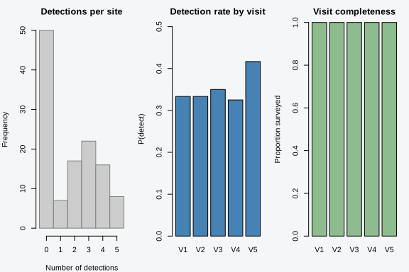
These summaries are a quick check that the reshape did what you meant. A visit column that is mostly empty, or a naive occupancy of zero, usually points to a site or visit id that did not line up during the reshape.
Missing visits
Sites are not always visited the same number of times. A site
surveyed three times in a five-visit design has two NA
entries in its row. The fitter handles this directly: each
NA becomes a missing marker internally, and the likelihood
sums only over the visits that were actually observed. No imputation, no
dropped sites.
y_miss <- y
y_miss[1, 4:5] <- NA   # site 1 surveyed 3 times
y_miss[2, 5]   <- NA   # site 2 surveyed 4 times
y_miss[1:3, ]
#>      [,1] [,2] [,3] [,4] [,5]
#> [1,]    0    0    1   NA   NA
#> [2,]    0    1    1    0   NA
#> [3,]    0    1    1    1    0
The fit runs unchanged on the gappy matrix, and the estimates stay close to the truth because the present visits still carry their information.
fit_miss <- tobs(
  ~ occ_cov1,
  data      = dat,
  family    = occu(),
  detection = ~ det_cov1,
  y         = y_miss,
  method    = "laplace",
  control   = list(verbose = FALSE)
)
coef(fit_miss)
#> psi_(Intercept)    psi_occ_cov1   p_(Intercept)      p_det_cov1
#>       0.3589342       0.9007435       0.3778563       0.5671907
A site with every visit missing is a special case: with no observations it contributes nothing to the detection likelihood, and under the spatial nested-Laplace engine it becomes a held-out site whose occupancy is interpolated from the latent field. The single-season Laplace fit simply carries it with no detection information.
Validation
tobs() checks the response shape before it builds
anything, so a malformed input fails with a named error rather than a
confusing fit failure several steps later. The two slips that catch
people are a wrong y type and a row-count mismatch between
y and data.
A single-season y must be a matrix. Passing a data frame
or a bare vector stops the build with the expected shape spelled
out.
tobs(~ occ_cov1, data = dat, family = occu(),
     detection = ~ det_cov1, y = as.data.frame(y),
     method = "laplace", control = list(verbose = FALSE))
#> Error in `.tobs_build_single()`:
#> ! y must be a matrix (n_sites x max_visits)
If the matrix has a different number of rows than data,
the error quotes both counts so you can see which side is wrong.
tobs(~ occ_cov1, data = dat[1:100, , drop = FALSE], family = occu(),
     detection = ~ det_cov1, y = y,
     method = "laplace", control = list(verbose = FALSE))
#> Error:
#> ! y has 120 rows but data has 100 rows
tobs_data() validates earlier, while it is still
reshaping the long frame. Naming a covariate column that is not in the
frame stops with the missing name quoted, before any matrix is
built.
tobs_data(long, y = "detected", site = "site", visit = "visit",
          occ.covs = "elevation")   # column is named 'elev', not 'elevation'
#> Error in `[.data.frame`:
#> ! undefined columns selected
The type argument is checked against the response
values. An occurrence response carrying a 2 is rejected,
since occurrence data is 0/1; an abundance response with a negative
count and a cover response outside [0, 1] fail the same way
against their own domains.
bad <- long
bad$detected[1] <- 2
tobs_data(bad, y = "detected", site = "site", visit = "visit",
          type = "occurrence")
#> Error in `.tobs_response_values()`:
#> ! tobs_data(type = 'occurrence'): y must be 0/1
The community and dynamic builders apply the matching check on their
own shapes. A dyn_occu() fit wants a 3D
[site x visit x season] array, and handing it a 2D matrix
reports the array requirement directly.
tobs(~ 1, data = dat, family = dyn_occu(), detection = ~ 1, y = y,
     colonization = ~ 1, extinction = ~ 1,
     method = "laplace", control = list(verbose = FALSE))
#> Error in `.tobs_build_dynamic()`:
#> ! y must be a 3D array [n_sites x max_visits x n_seasons] or a list of matrices
The pattern is the same across families: declare the site table and
the response, let the builder reconcile them, and read the error when
they do not match. When a fit refuses to start, checking
dim(y) against nrow(data) resolves most of it
before any inference runs.
Response shapes per family
The wide-matrix logic extends to the array and list families, and the
named elements stay constant: y holds the response,
occ.covs the per-site covariate frame,
det.covs the per-visit covariate matrices. Only the shape
of y moves. A single-season occu() or
abun() fit reads an N x J matrix; a community
ms_occu() or ms_abun() fit reads an
N x J x species array; a dynamic dyn_occu()
fit reads an N x J x season array; an integrated
int_occu() fit reads a list of matrices, one per source,
that may differ in their visit counts. The simulators are the fastest
way to see each shape, since they return a y already in the
form the matching family expects.
A community model stacks species on a third dimension.
simulate_ms_occu() returns an N x J x species
array, and species names that dimension.
sm <- simulate_ms_occu(N = 80, J = 4, n.species = 6, seed = 3)
dim(sm$y)   # sites x visits x species
#> [1] 80  4  6
An integrated model has one detection matrix per data source, with a
shared occupancy state across sources. simulate_int_occu()
returns y as a list of matrices that differ in their visit
counts.
si <- simulate_int_occu(N.total = 100, n.data = 2, J = c(4, 3),
                        n.shared = 20, seed = 42)
vapply(si$y, dim, integer(2))   # each source: sites x its own visit count
#>      [,1] [,2]
#> [1,]   60   60
#> [2,]    4    3
A dynamic model adds the season as a third dimension.
simulate_dyn_occu() returns an N x J x season
array, and the fit needs colonization and
extinction for the colonisation and extinction
processes.
sd <- simulate_dyn_occu(N = 60, J = 3, n.seasons = 4, seed = 1)
dim(sd$y)   # sites x visits x seasons
#> [1] 60  3  4
Each of those families has its own vignette that fits the model end to end. This one stops at the data shape, which is the part that is the same whether you go on to a Laplace fit or a full NUTS posterior.
See also
?tobs_data,?tobs_format,?tobs_format_msfor the constructors.The getting-started vignette for the fit, extract, and predict workflow.
The family vignettes (
vignette("community-models"),vignette("integrated-occupancy"),vignette("dynamic-occupancy")) for the array and list responses fit end to end.