Community models in tulpaObs • tulpaObs

Installation

install.packages("pak")
pak::pak("gcol33/tulpaObs")            # latest from GitHub
pak::pak("gcol33/tulpaObs@v0.1.1")     # a specific tagged release

Tagged releases are listed at https://github.com/gcol33/tulpaObs/releases.

pak resolves the dependency tree, pulling tulpa and tulpaMesh from the r-universe repository DESCRIPTION declares in Additional_repositories, at or above the Imports floor. A C++17 toolchain is needed (Rtools on Windows, Xcode CLI tools on macOS, r-base-dev on Linux); both tulpa and tulpaObs compile their backends on first install.

library(tulpaObs)

Why fit many species at once

A survey rarely records one species. You walk a transect, run a camera grid, or net a pond, and you come back with detections for dozens of taxa across the same sites and visits. The obvious move is to fit each species on its own: one occupancy model per species, one abundance model per species, stack the results. That works for the common species. It falls apart for the rare ones.

The rare species are where most of the data lives, in the sense that they are the majority of the species list and the minority of the detections. A bird seen at three sites out of two hundred carries almost no information on its own. Its single-species fit will have a slope with a credible interval running from deeply negative to deeply positive, an intercept pinned to the floor, and detection probability that the optimiser cannot separate from occupancy. You report it anyway, the interval covers everything, and the species adds nothing.

A community model changes the arithmetic. Instead of treating each species as an isolated problem, it assumes the species coefficients are draws from a shared distribution, a community. The mean of that distribution is estimated from every species jointly, and a species with thin data is pulled toward the community mean rather than left to drift. The pull is strongest where the data are weakest, which is exactly where you want it. A common species, well informed by its own detections, barely moves. A rare species, with nothing to anchor it, borrows the shape of the assemblage. This is partial pooling, and for assemblage data it is usually the difference between a species list you can interpret and a table of noise.

There is a second reason to fit the assemblage jointly, beyond rescuing the rare species. Many of the questions you ask of survey data are about the community, not about any one species. How many species occupy a site. How richness changes along a gradient. Whether the assemblage as a whole responds to disturbance. None of these has a single-species answer you can stack up afterward, because the uncertainty in each species’ contribution has to combine correctly into the community summary. A model that fits the species jointly carries that uncertainty through to the community quantity. A pile of separate fits does not, and the honest error bars on a richness map assembled from independent fits are hard to get right.

The same idea spans both response types tulpaObs supports for assemblages. ms_occu() fits community occupancy: presence-absence with imperfect detection, pooled across species. ms_abun() fits community N-mixture: repeated counts with a latent abundance per site, again pooled across species. The model structure is identical; only the per-species likelihood differs. This vignette builds both from simulated data with a known truth, reads the community means against that truth, pulls out species richness with its uncertainty, and ends with the rules of thumb for when pooling helps and when a single-species fit is the honest call.

The model

Write the coefficient vector for species $s$ as $\beta_s$ . In a single-species fit, each $\beta_s$ is a free parameter estimated only from species $s$ ’s data. A community model adds one layer above it: the species coefficients are themselves draws from a community distribution,

$\beta_s \;\sim\; \mathcal{N}(\mu,\; \Sigma),$

where $\mu$ is the community mean (the average response across the assemblage) and $\Sigma$ is the covariance of species around that mean. The community mean $\mu$ is the fixed effect: it is what coef() returns, and it is the quantity you interpret as “the typical response in this community”. The per-species departures $\beta_s - \mu$ are the random effects, the deviations that say how each species differs from the assemblage average.

For occupancy, $\beta_s$ holds the occupancy-arm coefficients (intercept and covariate slopes on the logit of $\psi$ ) and a parallel detection-arm vector with its own community mean and covariance. For the N-mixture, $\beta_s$ holds the abundance-arm coefficients on the log of $\lambda$ and the detection-arm coefficients on the logit of $p$ , each with its own community distribution. In both cases the latent state, occupancy $z$ in one and abundance $N$ in the other, integrates out, so the fit works directly with the marginal likelihood of the observed detections.

The detection arm pools just as the state arm does, and this is more than a symmetry of notation. Detection is the hardest thing to estimate per species, because a species seen rarely gives you almost no replicate detections to learn its detectability from. Pooling detection across the assemblage borrows the community’s detection mean for the species that cannot estimate their own, which is what keeps a rare species’ occupancy from being confounded with its detectability. The two arms have independent community distributions, so a species can be a detection outlier without being an occupancy outlier and the model keeps the two departures separate.

The width of $\Sigma$ controls how hard the pooling pulls. A narrow $\Sigma$ says species are alike, so a rare species is dragged close to $\mu$ . A wide $\Sigma$ says species are heterogeneous, so each keeps more of its own estimate. Crucially, $\Sigma$ is estimated from the data, not fixed by hand. The assemblage decides how much it resembles itself, and the pooling strength follows from that.

It helps to see the two extremes the community structure interpolates between. Fix $\Sigma$ at zero and every species collapses onto the community mean: this is complete pooling, a single coefficient for the whole assemblage that ignores species identity entirely. Let $\Sigma$ run to infinity and the prior tells each species nothing, so each $\beta_s$ is estimated from its own data alone: this is no pooling, the stack of independent single-species fits. The community model sits between, and because $\Sigma$ is fitted, the data choose where between. An assemblage of near-identical species lands near complete pooling; a heterogeneous one lands near no pooling. You do not pick the pooling strength, you let it be inferred, which is the difference between a defensible community fit and an arbitrary one.

The estimation works because the latent state never has to be sampled. In a naive formulation you would carry the occupancy indicators $z_{s,i}$ or the abundances $N_{s,i}$ as parameters and integrate them by simulation. tulpaObs instead sums them out in closed form, occupancy over the two states $z \in \{0,1\}$ and abundance over a truncated count range, so the likelihood the fitter sees is already marginal in the latent state. What remains are the per-species coefficients and their community distribution, and those are handled by a Laplace approximation at the mode with the community covariance updated from how the fitted species scatter. The result returns in well under a second on an assemblage of a few dozen species across a few hundred sites.

Community occupancy

simulate_ms_occu() draws an assemblage of occupancy histories with a known community truth. The community mean occupancy coefficients are beta.comm.mean (intercept and one covariate slope x), and species scatter around them with standard deviations beta.comm.sd. Here eight species share an occupancy intercept of 0 and a slope of 0.5, with species-level spread of 0.5 on the intercept and 0.3 on the slope.

sm <- simulate_ms_occu(N = 120, J = 5, n.species = 8, seed = 3)
dim(sm$y)            # 120 sites x 5 visits x 8 species
#> [1] 120   5   8
sm$truth$beta_comm_mean   # community occupancy intercept + slope on x
#> [1] 0.0 0.5
sm$truth$beta_comm_sd     # species-level SD around each community mean
#> [1] 0.5 0.3

The response y is a three-dimensional array: sites by visits by species. Each species occupies a slice sm$y[, , s], a sites-by-visits detection matrix of the same shape a single-species occu() would take. Stacking those slices is what turns eight occupancy models into one community fit. The detection histories vary a lot in how much they carry: the first species below is detected at many sites, a later one at only a handful, and the community prior is what keeps the sparse species from drifting.

detected <- apply(sm$y, 3, function(s) mean(rowSums(s, na.rm = TRUE) > 0))
round(setNames(detected, paste0("sp", 1:8)), 2)
#>  sp1  sp2  sp3  sp4  sp5  sp6  sp7  sp8 
#> 0.36 0.41 0.42 0.51 0.54 0.30 0.44 0.42

Fit with ms_occu(). The call shape is the single-species occupancy call with two additions: the response is the array, and species names the third dimension. The occupancy formula and the detection formula apply to every species; the community structure is what lets their coefficients differ.

fm <- tobs(
  ~ x,
  data      = sm$data,
  family    = ms_occu(),
  detection = ~ 1,
  y         = sm$y,
  species   = paste0("sp", 1:8),
  method    = "laplace",
  control   = list(verbose = FALSE)
)

coef() returns the community means, named by process. The psi_ coefficients are the community occupancy mean $\mu$ ; the p_ coefficients are the community detection mean. These are the assemblage-level fixed effects.

coef(fm)
#> psi_(Intercept)           psi_x   p_(Intercept) 
#>      -0.1803196       0.5286092      -0.3517980

Read the occupancy means against the truth. The simulated community intercept was 0 and the slope 0.5, and the fit lands close to both.

data.frame(
  term      = c("intercept", "slope_x"),
  estimate  = round(coef(fm, arm = "psi"), 3),
  truth     = sm$truth$beta_comm_mean,
  row.names = NULL
)
#>        term estimate truth
#> 1 intercept   -0.180   0.0
#> 2   slope_x    0.529   0.5

summary() adds the posterior standard deviation and credible bounds for each community mean. The psi_ rows are the occupancy community coefficients, the p_ row the detection one.

summary(fm)
#>                   estimate std.error      2.5 %      97.5 %
#> psi_(Intercept) -0.1803196 0.1257453 -0.4019536  0.07934851
#> psi_x            0.5286092 0.1486203  0.2400258  0.80830590
#> p_(Intercept)   -0.3517980 0.1339118 -0.6210877 -0.10140058

The credible bounds here are tight because they describe the community mean, which is informed by all eight species at once. A single species would report a far wider interval on the same slope. That narrowing is the pooling working: the assemblage estimates its average response sharply even though no individual species could.

The contrast is worth making concrete. Fit the sparsest species on its own with a single-species occu() and compare its slope to the community mean. The single-species interval is wide and may not even pin the sign; the community mean is sharp. The community fit does not make the sparse species’ own estimate sharper, it supplies a sharp assemblage average against which that species’ departure is small.

sparse_sp <- which.min(detected)        # the least-detected species
fit_one <- tobs(~ x, data = sm$data, family = occu(), detection = ~ 1,
                y = sm$y[, , sparse_sp], method = "laplace",
                control = list(verbose = FALSE))
rbind(
  single_species = round(confint(fit_one)["psi_x", ], 3),
  community_mean  = round(confint(fm)["psi_x", ], 3)
)
#>                 2.5 % 97.5 %
#> single_species -0.601  0.232
#> community_mean  0.240  0.808

The single-species slope carries an interval several times wider than the community mean’s. On a real survey, that single-species interval is what you would report species by species if you fit them separately, and most of them would say nothing. The community mean says something because it pooled.

Species richness

The reason to fit occupancy for a whole assemblage is often a single derived quantity: how many species occupy each site. The naive count, species detected at a site, understates richness because an occupied species can go undetected on every visit. The community model fixes this by carrying each species’ occupancy probability $\psi_{s,i}$ , so expected richness at site $i$ is the sum of occupancy probabilities across species, $\sum_s \psi_{s,i}$ , and the uncertainty in those probabilities propagates into the sum.

tobs_richness() does this from the fitted object. It returns a per-site table with the posterior mean richness, its standard deviation, and a 95% credible interval.

rich <- tobs_richness(fm)
head(rich)
#>   site     mean        sd     q2.5    q97.5
#> 1    1 2.685140 0.2592832 2.195456 3.201013
#> 2    2 3.342838 0.2216573 2.940087 3.780972
#> 3    3 3.915262 0.2841169 3.414729 4.521491
#> 4    4 2.514438 0.2827671 1.978909 3.097812
#> 5    5 3.850002 0.2737118 3.366689 4.430828
#> 6    6 3.677669 0.2494566 3.243775 4.195732

The column mean is the expected number of species present, summed over their occupancy probabilities rather than counted from detections. Because the sum runs over probabilities, it is a real number, not an integer: a site with five species each at $\psi = 0.6$ has expected richness 3.0. Plotting richness against site, ordered, shows the spread across the survey with its uncertainty band.

ord <- order(rich$mean)
r   <- rich[ord, ]
plot(seq_len(nrow(r)), r$mean, type = "n",
     xlab = "site (ordered by richness)", ylab = "expected richness",
     ylim = range(r$q2.5, r$q97.5))
polygon(c(seq_len(nrow(r)), rev(seq_len(nrow(r)))),
        c(r$q2.5, rev(r$q97.5)),
        col = adjustcolor("steelblue", 0.25), border = NA)
lines(seq_len(nrow(r)), r$mean, lwd = 2, col = "steelblue")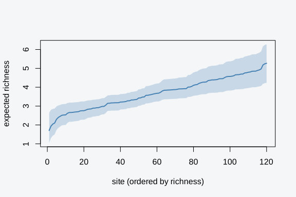

Estimated species richness per site, sorted, with a shaded 95 percent credible band

The band carries the occupancy uncertainty for every species into the richness estimate, so a site whose species are all marginally present reports both a lower richness and a wider interval than a site of confident occupants. That is the honest picture a raw detected-species count throws away.

It is worth seeing how far the estimate departs from the naive count. The naive richness at a site is the number of species detected there at least once; the modelled richness adds the species that are probably present but went undetected. The gap between them is the detection correction, and it grows with the number of visits a survey skipped and the species it would have caught with more effort.

naive <- rowSums(apply(sm$y, c(1, 3), function(v) any(v > 0, na.rm = TRUE)))
data.frame(
  site        = 1:6,
  detected    = naive[1:6],
  modelled    = round(rich$mean[1:6], 2),
  correction  = round(rich$mean[1:6] - naive[1:6], 2)
)
#>   site detected modelled correction
#> 1    1        3     2.69      -0.31
#> 2    2        3     3.34       0.34
#> 3    3        4     3.92      -0.08
#> 4    4        2     2.51       0.51
#> 5    5        2     3.85       1.85
#> 6    6        4     3.68      -0.32

The modelled richness exceeds the detected count at most sites, by the amount the model attributes to imperfect detection. A survey that visited each site five times misses less than one that visited twice, so the correction shrinks as visits accumulate. Reporting richness without this correction systematically undercounts, and the bias is worst exactly where detection is poor.

One note on what ms_occu() exposes. ranef() returns the per-species deviations from the community mean on both arms, occupancy (psi) and detection (p), the BLUPs the fitter places on each species and the same table shape ms_abun() returns below. tobs_richness() and fitted() give the per-species occupancy on the response scale; ranef() gives the deviations on the linear-predictor scale.

head(ranef(fm))
#>   arm   group level        term     estimate std.error
#> 1 psi species   sp1 (Intercept) -0.255318654        NA
#> 2 psi species   sp2 (Intercept)  0.008896697        NA
#> 3 psi species   sp3 (Intercept)  0.097276794        NA
#> 4 psi species   sp4 (Intercept)  0.190934586        NA
#> 5 psi species   sp5 (Intercept)  0.427014812        NA
#> 6 psi species   sp6 (Intercept) -0.373633186        NA

Community N-mixture

The count analogue is ms_abun(), the community version of Royle’s N-mixture. Each species has a latent abundance per site drawn from a Poisson with mean $\lambda_{s,i}$ , and the repeated visits are binomial detections of that abundance. The per-species abundance coefficients are drawn from a community Normal on the log scale, the detection coefficients from another on the logit scale, exactly the two-arm structure of the occupancy model with counts in place of presence.

simulate_ms_abun() draws this with a known community truth. The community abundance mean mu_lambda is on the log scale, so an intercept of $\log 3$ means the typical species averages three individuals per site at the covariate mean.

sab <- simulate_ms_abun(n.species = 8, N = 80, J = 4,
                        n.abund.covs = 1, n.det.covs = 1, seed = 7)
dim(sab$y)              # 80 sites x 4 visits x 8 species
#> [1] 80  4  8
sab$truth$mu_lambda     # community abundance mean (log scale): log(3), slope 0.4
#> [1] 1.098612 0.400000
sab$truth$mu_p          # community detection mean (logit scale)
#> [1]  0.3 -0.3

Fit with ms_abun(). The call mirrors the single-species abun() call, with the species array and species added.

fab <- tobs(
  ~ abund_cov1,
  data      = sab$data,
  family    = ms_abun(),
  detection = ~ det_cov1,
  y         = sab$y,
  species   = paste0("sp", 1:8),
  method    = "laplace",
  control   = list(verbose = FALSE)
)

coef() returns the community means: the lambda_ coefficients on the log scale, the p_ coefficients on the logit scale. The log link on the abundance arm matters for reading the intercept. A community abundance intercept near $\log 3 \approx 1.1$ back-transforms to about three individuals; do not read it as a count directly.

coef(fab)
#> lambda_(Intercept)  lambda_abund_cov1      p_(Intercept)         p_det_cov1 
#>          1.2540824          0.2358557          0.6379509         -0.4154767
exp(coef(fab, arm = "lambda")["(Intercept)"])   # community mean abundance at covariate mean
#> (Intercept) 
#>    3.504621

Compare the community means to the truth. The abundance arm is on the log scale, the detection arm on the logit scale.

data.frame(
  arm      = c("lambda", "lambda", "p", "p"),
  term     = c("intercept", "abund_cov1", "intercept", "det_cov1"),
  estimate = round(c(coef(fab, arm = "lambda"), coef(fab, arm = "p")), 3),
  truth    = round(c(sab$truth$mu_lambda, sab$truth$mu_p), 3),
  row.names = NULL
)
#>      arm       term estimate  truth
#> 1 lambda  intercept    1.254  1.099
#> 2 lambda abund_cov1    0.236  0.400
#> 3      p  intercept    0.638  0.300
#> 4      p   det_cov1   -0.415 -0.300

Per-species deviations

Where the community mean is the assemblage average, the per-species deviations say how each species departs from it. ranef() returns those deviations for an ms_abun fit, in long form: one row per species, arm, and term. The estimate is $\beta_s - \mu$ , the species’ offset from the community mean on the link scale.

re <- ranef(fab)
head(re, 8)
#>      arm   group level        term    estimate std.error
#> 1 lambda species   sp1 (Intercept)  0.01709827        NA
#> 2 lambda species   sp2 (Intercept) -0.20261975        NA
#> 3 lambda species   sp3 (Intercept) -0.14248986        NA
#> 4 lambda species   sp4 (Intercept)  0.13369841        NA
#> 5 lambda species   sp5 (Intercept)  0.39884530        NA
#> 6 lambda species   sp6 (Intercept) -0.27066324        NA
#> 7 lambda species   sp7 (Intercept)  0.01894771        NA
#> 8 lambda species   sp8 (Intercept)  0.08260407        NA

A positive abundance-intercept deviation marks a species more abundant than the community average, a negative one a sparser species. Pull the abundance-intercept deviations and order them into a caterpillar plot, the standard way to read random effects: species sorted by their offset, each a point against the community-mean line at zero.

dev_int <- re[re$arm == "lambda" & re$term == "(Intercept)", ]
dev_int <- dev_int[order(dev_int$estimate), ]
plot(dev_int$estimate, seq_len(nrow(dev_int)),
     yaxt = "n", pch = 19, col = "steelblue",
     xlab = "abundance-intercept deviation (log scale)", ylab = "",
     xlim = range(dev_int$estimate) + c(-0.1, 0.1))
axis(2, at = seq_len(nrow(dev_int)), labels = dev_int$species, las = 1)
abline(v = 0, lty = 2, col = "grey50")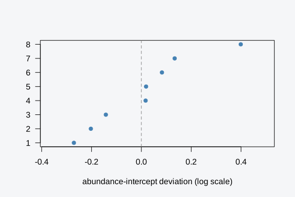

Caterpillar plot of per-species abundance-intercept deviations, ordered, against the community mean at zero

The community covariances $\Sigma_\lambda$ and $\Sigma_p$ sit on the fitted object as ms_community$sd_lambda and ms_community$sd_p, the per-coefficient community standard deviations. They report how heterogeneous the assemblage is around its mean, the estimated width of the community distribution that drove the pooling.

fab$ms_community$sd_lambda   # community SD of abundance coefficients
#> (Intercept)  abund_cov1 
#>   0.2076064   0.6141322
fab$ms_community$sd_p        # community SD of detection coefficients
#> (Intercept)    det_cov1 
#>   0.3573648   0.5066321

A small community SD says the species behave alike, so the pooling pulled rare species hard toward the mean. A large one says they are heterogeneous, so each species kept more of its own estimate. Reading the SD alongside the deviations tells you how much work the community prior is doing.

The per-species coefficients themselves, community mean plus deviation, give the per-species abundance you would predict at the covariate mean. Back-transform the abundance intercept of each species through exp() to read it as a count, and the spread across species shows the assemblage from sparse to abundant.

coef_lambda <- fab$ms_community$coef_lambda          # one row per species
per_species_N <- round(exp(coef_lambda[, "(Intercept)"]), 2)
sort(per_species_N)
#>  sp6  sp2  sp3  sp1  sp7  sp8  sp4  sp5 
#> 2.67 2.86 3.04 3.57 3.57 3.81 4.01 5.22

These are the species-level estimates the community structure produced. A sparse species’ value is close to the community mean because the pooling supplied most of it; an abundant species with ample counts sits at its own data. The community SD above is what set how far each was allowed to stray.

ms_abun() fits a community N-mixture under method = "laplace" – Poisson by default, or negative-binomial with mixture = "negbin". The NB arm gives each species its own overdispersion through a log-normal random effect (log r_s ~ N(mu_log_r, sigma_log_r)), so the dispersion is partially pooled across the assemblage the same way the coefficients are; fit$ms_dispersion returns the per-species r_s alongside the community mu_log_r and sigma_log_r. For a single overdispersed species on its own, abun(mixture = "negbin") covers that case directly (see vignette("abundance")).

Per-species overdispersion

Counts in the wild are rarely Poisson. A site that suits a species holds a cluster; an unsuitable one holds none, and the variance of the counts outruns their mean. The Poisson abundance arm has no room for that, so an overdispersed species inflates the detection estimate to soak up the extra variance and the abundance mean drifts. mixture = "negbin" gives each species its own negative-binomial size $r_s$ , with the per-species log-dispersions drawn from a community Normal, $\log r_s \sim \mathcal{N}(\mu_{\log r}, \sigma_{\log r}^2)$ . The dispersion pools across the assemblage the same way the coefficients do: a species with thin counts borrows the community log-dispersion, a species with many counts keeps its own.

Simulate an assemblage with genuine overdispersion. size = 5 sets the community-mean size (so $\mu_{\log r} = \log 5$ ), and sigma.logr = 0.5 spreads the per-species sizes around it. Eight species over 80 sites with four visits keep the example quick while still letting per-species dispersion register.

snb <- simulate_ms_abun(n.species = 8, N = 80, J = 4,
                        n.abund.covs = 1, n.det.covs = 1,
                        mu.lambda = c(log(5), 0.4), mu.p = c(0.3, -0.3),
                        sd.lambda = 0.4, sd.p = 0.35,
                        mixture = "negbin", size = 5, sigma.logr = 0.5,
                        seed = 14)
snb$truth$mu_log_r          # community log-dispersion: log(5)
#> [1] 1.609438
snb$truth$sigma_log_r       # spread of per-species log r
#> [1] 0.5

Fit with ms_abun(mixture = "negbin"). The call is the Poisson community call with the mixture switched. The per-species RE vector widens by one coordinate for log_r_s, so the AGHQ grid grows; control$n.quad = 2 keeps it small without losing the small-cluster correction.

fnb <- tobs(
  ~ abund_cov1,
  data      = snb$data,
  family    = ms_abun(mixture = "negbin"),
  detection = ~ det_cov1,
  y         = snb$y,
  species   = snb$species,
  method    = "laplace",
  control   = list(verbose = FALSE, n.quad = 2L)
)
fnb$mixture
#> [1] "negbin"

The community log-dispersion sits on fit$ms_dispersion, alongside the per-species sizes r_s and the community spread sigma_log_r. mu_log_r is the assemblage-mean log size; $\exp(\mu_{\log r})$ is the size of the typical species.

disp <- fnb$ms_dispersion
c(mu_log_r    = round(disp$mu_log_r, 3),
  sigma_log_r = round(disp$sigma_log_r, 3),
  r_community = round(disp$r, 3))
#>    mu_log_r sigma_log_r r_community 
#>       1.640       0.362       5.157

Read the community log-dispersion against its truth. mu_log_r enters the coefficient surface as log_r, so its standard error is on fit$sds, and the estimate lands within a couple of standard errors of $\log 5$ .

data.frame(
  quantity  = c("mu_log_r", "sigma_log_r"),
  estimate  = round(c(disp$mu_log_r, disp$sigma_log_r), 3),
  truth     = round(c(snb$truth$mu_log_r, snb$truth$sigma_log_r), 3),
  row.names = NULL
)
#>      quantity estimate truth
#> 1    mu_log_r    1.640 1.609
#> 2 sigma_log_r    0.362 0.500

A community fit gains more from per-species dispersion than a single-species one does. The negative binomial carries variance $\lambda + \lambda^2 / r_s$ , so a small $r_s$ lets a species’ counts spread well beyond their mean without forcing the detection probability down to absorb the slack. Under a shared Poisson the clumped species would each push the community detection mean low, and the rare species, leaning on that mean, would inherit the bias. Pooling the dispersion keeps the overdispersion where it belongs, on the abundance arm, species by species, so the detection community mean stays clean for the species that depend on it.

The per-species sizes are in disp$r_s, one per species. A small $r_s$ marks a clumped species whose counts vary far more than their mean; a large one approaches the Poisson limit. The deviations behind them reach ranef() as a logr arm, the per-species $\log r_s - \mu_{\log r}$ on the same scale the coefficient deviations use.

re_nb <- ranef(fnb)
head(re_nb[re_nb$arm == "logr", ], 6)
#>     arm   group level  term    estimate std.error
#> 33 logr species   sp1 log_r -0.07748425        NA
#> 34 logr species   sp2 log_r  0.19427529        NA
#> 35 logr species   sp3 log_r  0.37531448        NA
#> 36 logr species   sp4 log_r -0.49715641        NA
#> 37 logr species   sp5 log_r  0.04376571        NA
#> 38 logr species   sp6 log_r  0.22623248        NA

Plot the per-species sizes with a band for the community spread. The points are each species’ fitted $r_s$ , sorted; the dashed line is the community-mean size $\exp(\mu_{\log r})$ , and the shaded band spans $\exp(\mu_{\log r} \pm \sigma_{\log r})$ , the central interval the community distribution places on a new species.

rs   <- sort(disp$r_s)
band <- exp(disp$mu_log_r + c(-1, 1) * disp$sigma_log_r)
plot(seq_along(rs), rs, pch = 19, col = "steelblue", log = "y",
     xlab = "species (ordered by size)", ylab = expression(r[s]~"(log axis)"),
     panel.first = rect(0, band[1], length(rs) + 1, band[2],
                        col = adjustcolor("steelblue", 0.15), border = NA))
abline(h = disp$r, lty = 2, col = "grey40")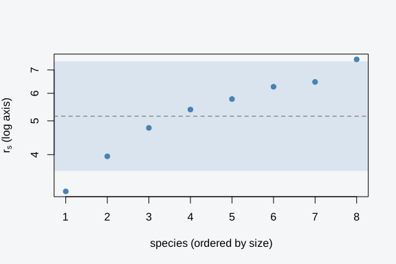

Per-species negative-binomial size r_s, sorted, against the community-mean size and its one-SD band

A species sitting below the band is more overdispersed than the assemblage typically is; one above it is closer to Poisson. The species that fall inside the band are the ones whose own counts told the model little, so the community log-dispersion supplied most of their size. With sigma.logr = 0 the simulator would give a single shared $r$ and every point would land on the line; the spread here is the assemblage genuinely differing in how clumped its species are.

Reading community against species-level effects

The two scales a community model reports answer different questions, and keeping them straight is the whole point of the structure.

The community mean from coef() answers “what is the typical response across this assemblage”. Its credible interval is narrow because every species informs it. This is the right number for a statement about the community as a whole: the assemblage occupies sites more often where x is high, the typical species averages three individuals per site.

The per-species coefficients answer “how does this particular species respond”. For both families they are the community mean plus the ranef() deviation; for ms_occu() the per-species occupancy probabilities also come on the response scale through fitted() and tobs_richness(). A rare species’ per-species estimate sits close to the community mean precisely because the model could not learn much from its own data and leaned on the assemblage. Read its credible interval, not just its point, and remember that the point is partly borrowed.

The mistake to avoid is reading a shrunk per-species estimate as if it were an independent measurement. A rare species pulled to the community mean has not told you it resembles the assemblage; the model has assumed it does and supplied the rest. The community SD on the fitted object is the honest measure of how much that assumption was allowed to matter. When the SD is wide, the pooling is gentle and the per-species estimates are mostly their own; when it is narrow, the rare species are mostly the community mean wearing a species label.

This is also why the community mean and the per-species deviations should be read together rather than in isolation. The deviation ranef() reports is a departure from a mean that the same fit estimated, so a deviation of zero means “this species behaves like the assemblage”, not “this species has no effect”. A species whose deviation interval covers zero is consistent with the community average, and for a rare species that consistency is largely the prior speaking. The deviations that carry information are the ones that pull clear of zero despite the shrinkage, because those species had enough of their own data to resist the pull.

Practical guidance

A few rules of thumb for community fits, with the numbers that make them actionable.

At least 8 to 10 species before pooling pays. The community mean and covariance are learned from how species scatter, and a handful of species leaves $\Sigma$ barely informed. Below roughly five species, the community prior is mostly your assumption rather than the data’s, and separate single-species fits are the more honest report. The pooling repays its machinery when you have dozens of species, many of them rare.
Sites in the dozens to hundreds. Each species still needs enough sites for its own signal to register before the community can refine it. With fewer than about 20 sites, even the common species are weakly estimated and the community mean inherits that weakness. The community model borrows strength across species; it does not manufacture it from nothing.
Pooling helps most for the rare species, least for the common ones. A species detected at 5% of sites gains the most from the community mean; a species detected at half its sites barely moves. If your question is only about the abundant species, the community structure adds machinery for little gain, and a single-species fit on each is simpler to defend.
A single-species fit is the honest choice when one species is the question. If you care about one focal species and have ample data on it, fit it alone with occu() or abun(). Borrowing from an assemblage you do not care about only muddies a clean estimate, and the community mean is irrelevant to a single-species inference.
When not to pool: heterogeneous assemblages. If the species genuinely do not share a response, a generalist and a specialist responding to opposite ends of a gradient, the community Normal is the wrong model and will fight the data. A wide fitted community SD is the warning sign: the assemblage is telling you it does not resemble itself, and the pooling is buying little. In that case the community mean is an average over species that have no common centre, and it describes none of them.
Check the community SD before trusting a shrunk estimate. The fitted ms_community$sd_lambda and sd_p (or the occupancy community SD reported in the fit) are the single most useful diagnostic. A community SD near zero on a coefficient means the model decided the species are interchangeable on that axis, and every per-species estimate there is essentially the community mean. That is fine when it is true and misleading when it is not, so confirm it against what you know of the natural history before reporting per-species effects on a near-zero-SD axis.

The pattern under all five rules is the same. The community model trades per-species independence for assemblage-level precision, and the trade is worth making when the species inform each other and a waste when they do not. The fitted community SD is where the model tells you which case you are in, and reading it is the habit that separates a community fit you can defend from one that merely produced numbers.

The community engine

The community families fit under method = "laplace"; every one of them except ms_distance() also takes method = "nuts", ms_occu(), ms_dyn_occu(), jsdm(), ms_count(), ms_abun() and ms_distance() take method = "nested_laplace" for a shared field, and ms_occu(), ms_dyn_occu(), ms_int_occu(), jsdm() and ms_count() take method = "pg_gibbs". Each Laplace fit is driven by one community Laplace-EM: per species the latent state integrates out in closed form, the per-species coefficient deviations are integrated by a joint-Newton mode-find with the random-effect blocks folded out by a Schur complement, and a closed-form M-step updates the per-arm community covariance. The occupancy and detection deviations are independent, each with its own covariance $\Sigma$ , so a species’ occupancy departure and its detection departure are estimated separately rather than tied together. Community-mean standard errors come from the marginal observed information at the mode (the Schur complement of the random-effect block). The fit finds the posterior mode and the curvature there and returns in a fraction of a second.

The community N-mixture ms_abun() runs the same way; both its Poisson and negative-binomial arms use that one engine, the NB through the AGHQ path that integrates the per-species log-dispersion. A gradient sampler for the community families is not offered: a correct community posterior needs independent per-arm random-effect blocks in the sampler, which the shared HMC path does not yet carry.

Where to go next

Single-season occupancy end to end: vignette("occupancy").
N-mixture abundance, negative binomial, and areal spatial counts: vignette("abundance").
Random effects with lme4 bar syntax, the single-species analogue of community pooling: vignette("random-effects").
Posterior-predictive checks and WAIC for model comparison: vignette("diagnostics"). ```