Installation
install.packages("pak")
pak::pak("gcol33/tulpaObs")            # latest from GitHub
pak::pak("gcol33/tulpaObs@v0.1.1")     # a specific tagged release
Tagged releases are listed at https://github.com/gcol33/tulpaObs/releases.
pak resolves the dependency tree, pulling tulpa and
tulpaMesh from the r-universe repository DESCRIPTION
declares in Additional_repositories, at or above the
Imports floor. A C++17 toolchain is needed (Rtools on
Windows, Xcode CLI tools on macOS, r-base-dev on Linux);
both tulpa and tulpaObs compile their backends
on first install.
When a grouping factor needs a random effect
Surveys come with structure that is not a covariate of interest. Sites fall into clusters, observers differ in how hard they look, regions sit under their own unmeasured baseline. You could enter the grouping factor as a fixed effect, one coefficient per level, and for a handful of levels that is fine. With thirty observers or two hundred site clusters it stops being fine: each level gets its own intercept estimated from its own sparse data, the levels with little data get wild estimates, and nothing ties them together.
A random effect ties them together. Instead of estimating each level freely, you assume the level effects are draws from a common distribution, , and estimate the spread . A level with plenty of data keeps most of its own signal; a level with little data is pulled toward the population mean. The model spends one parameter on the spread rather than one per level, and the per-level estimates borrow strength from each other. This is the difference between asking “what is this observer’s intercept” and “how much do observers vary, and where does this one sit”.
The honest question to ask first is which one you want. If the
grouping factor has a few levels and each is interesting in its own
right (three treatment arms, two field protocols), a fixed effect names
them and is the right tool. If it has many exchangeable levels and you
care about the variance more than any single level, a random effect is
the right tool. tulpaObs writes random effects the way lme4
does, inside the formula, with a bar.
The pull toward the mean is called shrinkage, and it is the feature, not a side effect. A cluster surveyed once contributes one noisy observation; on its own that observation would give a wild intercept. The random effect treats it as a draw from the population and reports an estimate close to the population mean, because the data give little reason to move it. A cluster surveyed two hundred times anchors its own estimate, because its data dominate the prior. The amount of shrinkage is set by the data, not chosen: it falls out of the ratio between within-group noise and the estimated between-group variance . This is also why a random effect reports honest uncertainty. A fixed effect with one observation per level claims a precise intercept it has no right to; the random effect admits it is mostly guessing the mean.
Bar syntax
A random-effect term is
(<effects> | <grouping factor>). The left side
says which coefficients vary by group; the right side names the grouping
factor (a factor in your data frame). The double bar
|| drops the correlation between a group’s intercept and
its slopes. The supported forms:
| Form | Meaning |
|---|---|
(1 | g) |
random intercept per level of g
|
(x | g) |
random intercept and slope on x, correlated |
(1 + x | g) |
the same, written explicitly |
(x || g) |
random intercept and slope, uncorrelated |
(1 + x || g) |
the same, written explicitly |
(0 + x | g) |
random slope on x, no group intercept |
(1 | g:h) |
random intercept for each crossed combination of g and
h
|
(1 | g/h) |
nested: a g intercept plus an
h-within-g intercept |
A term enters whichever linear predictor its formula sits in. Put
(1 | g) in the occupancy formula and it varies occupancy by
group; put it in the detection formula and it varies
detection by group. The process membership comes from the formula, not
from a separate argument.
Under the hood tulpaObs rewrites the bars into
re() calls on the formula tree before parsing, so there is
one parser and one term type. You never call re() yourself;
the bar is the surface you type.
A random intercept under Laplace
Start with the simplest case: occupancy varies by a site cluster. We
simulate thirty clusters of twenty-five sites each, give each cluster
its own intercept drawn from
,
and add one site covariate x. Detection is constant at
about 0.45 across six visits.
sim_re <- function(seed = 101, ng = 30L, per = 25L, J = 6L,
                   b0 = 0.3, b1 = -0.6, sigma = 0.9, p = 0.45) {
  set.seed(seed)
  N <- ng * per
  g <- rep(seq_len(ng), each = per)
  x <- rnorm(N)
  b_true <- rnorm(ng, 0, sigma)               # the per-cluster intercepts
  z <- rbinom(N, 1, plogis(b0 + b1 * x + b_true[g]))
  y <- matrix(0L, N, J)
  for (i in seq_len(N)) y[i, ] <- rbinom(J, 1, z[i] * p)
  list(y = y, d = data.frame(g = factor(g), x = x), b_true = b_true)
}

s <- sim_re()
str(s$d)
#> 'data.frame':    750 obs. of  2 variables:
#>  $ g: Factor w/ 30 levels "1","2","3","4",..: 1 1 1 1 1 1 1 1 1 1 ...
#>  $ x: num  -0.326 0.552 -0.675 0.214 0.311 ...
The grouping factor g is a factor. Fit
occupancy with a fixed slope on x and a random intercept
for g. The default method = "laplace" fits the
random effect through a variance-component EM; pass
verbose = FALSE so the EM does not print its
iterations.
fit <- tobs(
  ~ x + (1 | g),
  data      = s$d,
  y         = s$y,
  detection = ~ 1,
  family    = occu(),
  method    = "laplace",
  control   = list(verbose = FALSE)
)
The fixed effects come back from coef() as usual. The
occupancy intercept and slope land near the simulated 0.3 and -0.6.
coef(fit, arm = "psi")
#> (Intercept)           x
#>   0.2369320  -0.6833076
The variance component is a hyperparameter in fit$means,
named for the group it belongs to. There is one sigma_
entry for the random intercept.
sig_name <- grep("^sigma_", names(fit$means), value = TRUE)
sig_name
#> [1] "sigma_g1_(Intercept)"
c(estimate = fit$means[[sig_name]], truth = 0.9)
#>  estimate     truth
#> 0.7309166 0.9000000
ranef() returns the per-group effects (the BLUPs, best
linear unbiased predictors) as a data frame with one row per group and
term: which arm the effect enters, which grouping factor, which level,
which coefficient, the estimate, and its standard error. Every family
returns these same columns.
re <- ranef(fit)
head(re)
#>   arm group level        term   estimate std.error
#> 1 psi     g     1 (Intercept) -0.3783381 0.3687621
#> 2 psi     g     2 (Intercept)  0.4034067 0.3834248
#> 3 psi     g     3 (Intercept)  0.6410361 0.3966751
#> 4 psi     g     4 (Intercept)  0.6755256 0.3915525
#> 5 psi     g     5 (Intercept) -0.2302246 0.3732743
#> 6 psi     g     6 (Intercept) -1.0928680 0.3860100
nrow(re)
#> [1] 30
The point of the random effect is that these per-cluster intercepts track the truth. Plotting the recovered BLUPs against the simulated cluster effects shows the model recovers the cluster-level signal, with the shrinkage that pulls small-data clusters toward zero.
plot(s$b_true, re$estimate, pch = 16, col = rgb(0, 0, 0, 0.5),
     xlab = "true cluster effect", ylab = "estimated BLUP")
abline(0, 1, col = "steelblue", lwd = 2)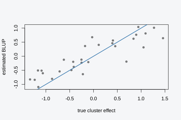
cor(s$b_true, re$estimate)
#> [1] 0.8786531
The EM, the small-cluster bias, and the AGHQ debias
The default Laplace path integrates the random-effect block with a
Gaussian approximation at its mode. For binary occupancy data that is
the glmer nAGQ = 1 regime: the per-group
integral is approximated by a single Gaussian, and at small per-group
sample sizes that approximation pulls the estimated variance toward
zero. The point estimates and the fixed-effect standard errors are fine;
the variance component itself comes out attenuated.
tulpaObs corrects this by default with an adaptive Gauss-Hermite
quadrature pass. After the EM converges it replaces the single-Gaussian
per-group integral with a quadrature grid, which captures the curvature
the Laplace approximation misses, and re-estimates the variance
component. The control is re.aghq (on by default) and
n.quad (the number of quadrature nodes, default 9). The fit
records what happened in fit$aghq.
fit$aghq$applied
#> [1] TRUE
fit$aghq$n_quad
#> [1] 9
The effect is largest when groups are small. With per-group the measured sigma bias runs about 18% under the raw EM and drops to about 4% after the AGHQ pass, matching a NUTS fit. We can see the direction on a single small-cluster dataset by turning the pass off and on.
s8 <- sim_re(seed = 21, ng = 30L, per = 8L, sigma = 0.9)

fit_em <- tobs(~ x + (1 | g), data = s8$d, y = s8$y, detection = ~ 1,
               family = occu(), method = "laplace",
               control = list(re.aghq = FALSE, verbose = FALSE))
fit_aghq <- tobs(~ x + (1 | g), data = s8$d, y = s8$y, detection = ~ 1,
                 family = occu(), method = "laplace",
                 control = list(re.aghq = TRUE, verbose = FALSE))

get_sigma <- function(f) f$means[[grep("^sigma_", names(f$means), value = TRUE)]]
c(truth = 0.9,
  EM    = get_sigma(fit_em),
  AGHQ  = get_sigma(fit_aghq))
#>     truth        EM      AGHQ
#> 0.9000000 0.5597824 0.6318479
The EM estimate sits below the truth; the AGHQ pass corrects it
upward. The mechanism is worth one sentence: a single Gaussian centred
at the per-group mode underweights the tails of the integral over the
group effect, and for binary data that loss falls on the variance, so
the estimate shrinks. Adding quadrature nodes samples those tails and
recovers the spread. You rarely need to think about this. The default
does the right thing, and fit$aghq$applied tells you it
ran. The pass applies to one grouping factor on one predictor with
random-effect dimension up to 3; outside that (a random effect split
across both occupancy and detection, crossed or nested groupings) the
fit keeps the EM estimate, and NUTS is available for the full
treatment.
Correlated random slopes
A random slope lets the covariate effect vary by group, not just the
intercept. (1 + x | g) gives each group its own intercept
and its own slope on x, with a correlation between the two
estimated as well. We simulate from a known
covariance with a positive intercept-slope correlation.
sim_corr <- function(seed = 402, ng = 40L, per = 25L, J = 6L,
                     b0 = 0.2, b1 = -0.4, p = 0.5,
                     Sigma = matrix(c(0.6, 0.3, 0.3, 0.4), 2, 2)) {
  set.seed(seed)
  N <- ng * per
  g <- rep(seq_len(ng), each = per)
  x <- rnorm(N)
  U <- matrix(rnorm(ng * 2L), ng, 2L) %*% chol(Sigma)   # rows ~ N(0, Sigma)
  eta <- b0 + U[g, 1] + (b1 + U[g, 2]) * x
  z <- rbinom(N, 1, plogis(eta))
  y <- matrix(0L, N, J)
  for (i in seq_len(N)) y[i, ] <- rbinom(J, 1, z[i] * p)
  list(y = y, d = data.frame(g = factor(g), x = x), U = U, Sigma = Sigma)
}

sc <- sim_corr()
fit_c <- tobs(~ x + (1 + x | g), data = sc$d, y = sc$y, detection = ~ 1,
              family = occu(), method = "laplace",
              control = list(verbose = FALSE))
The block reports two standard deviations (one for the intercept, one
for the slope) and the off-diagonal as a correlation named
cor_<g>_.... The true correlation here is
.
fit_c$means[grep("^sigma_|^cor_", names(fit_c$means))]
#> sigma_g1_(Intercept)           sigma_g1_x cor_g1_(Intercept)_x
#>            0.8249986            0.7169608            0.7626199
The Laplace correlation is regularized by a default
LKJ()
penalty (re.lkj) on each correlated block. A random-effect
correlation is often weakly identified, and unregularized maximum
likelihood can pin it against
.
The LKJ penalty pulls a weakly-identified correlation off the boundary
toward zero without touching the marginal standard deviations. Set
re.lkj = 1 to disable it; for a full posterior treatment of
the correlation, use NUTS.
The per-group slopes recover too. The ranef() table now
carries both an (Intercept) term and an x term
per group.
re_c <- ranef(fit_c)
unique(re_c$term)
#> [1] "(Intercept)" "x"
b1_hat <- re_c$estimate[re_c$term == "x"]
cor(b1_hat, sc$U[, 2])
#> [1] 0.8839711
The uncorrelated forms (x || g),
(1 + x || g), and the slope-only (0 + x | g)
fit the same way; they drop the off-diagonal, so you get the standard
deviations without a cor_ entry. Use || when
you have no reason to expect the intercept and slope deviations to move
together, or when the correlation is too weakly informed to
estimate.
Crossed and nested grouping
Two grouping factors can apply at once. They are crossed when every
level of one can pair with every level of the other (sites visited by
any of several observers), and nested when each level of the inner
factor belongs to exactly one level of the outer (transects within
plots). The bar syntax follows lme4: (1 | g:h)
is crossed, (1 | g/h) is nested.
Crossed grouping builds one random intercept for each observed combination of the two factors. We cross eight site groups with six survey rounds and give each combination its own occupancy intercept.
set.seed(55)
ng <- 8L; nh <- 6L; per <- 12L
combos <- expand.grid(g = seq_len(ng), h = seq_len(nh))
N <- nrow(combos) * per
g <- rep(combos$g, each = per); h <- rep(combos$h, each = per)
gh <- interaction(factor(g), factor(h), drop = TRUE)
b_gh <- rnorm(nlevels(gh), 0, 0.8)
x <- rnorm(N)
z <- rbinom(N, 1, plogis(0.2 - 0.4 * x + b_gh[gh]))
y <- matrix(0L, N, 6L)
for (i in seq_len(N)) y[i, ] <- rbinom(6L, 1, z[i] * 0.5)
d_cr <- data.frame(g = factor(g), h = factor(h), x = x)

fit_cr <- tobs(~ x + (1 | g:h), data = d_cr, y = y, detection = ~ 1,
               family = occu(), method = "laplace",
               control = list(verbose = FALSE))
nrow(ranef(fit_cr))      # one BLUP per observed g:h combination
#> [1] 48
coef(fit_cr, arm = "psi")
#> (Intercept)           x
#>   0.3424996  -0.5272869
The crossed term (1 | g:h) collapses to a single
interaction factor, so the Laplace path treats it as one grouping factor
and the AGHQ debias applies. The nested form (1 | g/h)
expands to two terms, an outer g intercept and an inner
h-within-g intercept; the EM fits both, and
the AGHQ debias steps aside because there is more than one grouping
factor. Read the nested variance components as the attenuated EM
estimates, or refit under NUTS when the variance partition matters.
A random effect on detection
Detection effort varies by observer. Put the bar in the
detection formula and the random effect moves the detection
probability instead of occupancy. Here observers each have their own
detection intercept, drawn from
,
while occupancy depends on a site covariate with no random part.
sim_det <- function(seed = 1, N = 400L, J = 6L, ng = 40L,
                    b0 = 0.4, b1 = -0.7, d0 = 0.2, sigma = 0.8) {
  set.seed(seed)
  occ_cov  <- rnorm(N)
  observer <- sample.int(ng, N, replace = TRUE)
  b_obs    <- rnorm(ng, 0, sigma)
  z <- rbinom(N, 1, plogis(b0 + b1 * occ_cov))
  p <- plogis(d0 + b_obs[observer])
  y <- matrix(0L, N, J)
  for (i in seq_len(N)) if (z[i] == 1L) y[i, ] <- rbinom(J, 1L, p[i])
  list(y = y, d = data.frame(occ_cov = occ_cov, observer = factor(observer)),
       b_obs = b_obs)
}

sd_re <- sim_det()
fit_d <- tobs(~ occ_cov, detection = ~ (1 | observer), family = occu(),
              data = sd_re$d, y = sd_re$y, method = "laplace",
              control = list(verbose = FALSE))
The variance component now belongs to the detection arm, so it is
named for the detection process: sigma_p<t>_ rather
than the occupancy sigma_g<t>_. The AGHQ pass records
that it ran on the detection arm.
grep("^sigma_", names(fit_d$means), value = TRUE)
#> [1] "sigma_p1_(Intercept)"
fit_d$aghq$arm
#> [1] "det"
The detection arm is harder than the occupancy arm because only occupied sites carry information about detection. A site that is empty tells you nothing about how well the observer detects. The raw EM attenuates the detection-RE variance heavily for that reason (about 70% in the measured sims), and the AGHQ pass on the exact detection marginal restores it to within about 1% with 88-96% fixed-effect interval coverage. The per-group detection BLUPs track the simulated observer effects.
Laplace versus NUTS for random effects
The Laplace path with the AGHQ debias covers the common single-grouping cases: a random intercept or slope on one of the two predictors, with the variance component corrected for the small-cluster bias. NUTS fits every random-effect form and returns the full posterior, including the full posterior of the correlation rather than a regularized point estimate. It is the tool for the forms Laplace declines and for any case where you want draws rather than a Gaussian approximation.
Here is the same random intercept under NUTS. The variance component
is reported on the natural scale under the same sigma_ name
the Laplace fit uses, and ranef() reconstructs the
per-group BLUPs by marginalising over the draws.
fit_n <- tobs(~ x + (1 | g), data = s$d, y = s$y, detection = ~ 1,
              family = occu(), method = "nuts",
              control = list(n.iter = 400, n.warmup = 200, seed = 1,
                             verbose = FALSE))

sig_l <- fit$means[[grep("^sigma_", names(fit$means), value = TRUE)]]
sig_n <- fit_n$means[[grep("^sigma_", names(fit_n$means), value = TRUE)]]
c(laplace = sig_l, nuts = sig_n, truth = 0.9)
#>   laplace      nuts     truth
#> 0.7309166 0.7792917 0.9000000
The two backends agree on the variance, and the BLUPs agree across engines.
Two random-effect specifications are NUTS-only. The Laplace path
errors, with a pointer to NUTS, for: a single random effect shared
across both the occupancy and detection predictors (share()
semantics), and a random effect combined with a spatial field in the
same fit. In each case the deterministic path would have to fit
something it cannot represent exactly, so it stops rather than silently
fitting a different model. NUTS handles both. A random effect beside
visit-level detection covariates, or one grouped over visit rows, stays
on the Laplace path: the detection arm is then fitted per (site, visit)
row, and only the AGHQ debias declines, so the variance components are
the EM values.
The reason for the boundary is in how the Laplace path works. The
variance-component EM splits the random effects into an occupancy arm
and a detection arm by which predictor they sit in, then fits each arm’s
block separately while feeding its mode back into the other process. A
single effect that has to be the same realization in both predictors
breaks that split: there is no way to fit it once on the occupancy arm
and once on the detection arm and call the two the same. Likewise the
AGHQ debias works on a per-site marginal with the latent occupancy state
integrated out in closed form; a spatial field changes that marginal in
a way the closed form does not cover, and a per-visit detection design
couples every visit of a site so the integrand no longer factors by
group. The first stops the fit; the second only switches the debias off.
Rather than approximate silently, the validator names NUTS, which
samples the joint posterior directly and needs none of these closed
forms. The cost is speed: a NUTS fit takes seconds where Laplace takes a
fraction of one, and you read convergence from Rhat and
effective sample size rather than trusting a mode.
Practical guidance
- Want at least five to eight levels before the variance is informed. A random effect estimates the spread across levels. With two or three levels there is almost no information about that spread, the variance is badly determined, and a fixed effect that names each level is the honest choice. Five to eight levels is the rough floor where the variance starts to mean something; the recovery here used thirty and forty.
- Use a fixed effect when the levels are few and each is interesting. Treatment arms, field protocols, a handful of named regions: these are fixed effects. You want their individual values, not their variance, and there are too few to estimate a variance well.
- Keep at least ten or so observations per group for slopes. A random slope asks each group’s data to inform its own slope before shrinkage. Groups with two or three observations contribute almost nothing and the block leans entirely on the population estimate. Random intercepts tolerate sparser groups than random slopes do.
-
Trust the AGHQ default on small clusters. When
per-group counts drop below about ten, the raw EM variance is
attenuated; the default
re.aghq = TRUEcorrects it. Checkfit$aghq$appliedto confirm it ran. When it does not apply (split arms, crossed or nested groupings, RE dimension above 3), read the variance as a lower bound and refit under NUTS if the variance matters to your conclusion. -
Reach for
||when the correlation is not the point. The correlated block(1 + x | g)spends a parameter on the intercept-slope correlation, which is often weakly identified. If you have no use for that correlation,(x || g)drops it and estimates the two standard deviations more stably. - When not to use a random effect at all. If the grouping factor is the exposure you care about (the thing whose effect is your research question), it belongs in the fixed part of the model. A random effect is for nuisance structure you want to account for, not for the signal you came to measure.
Where to go next
- The single-season occupancy model the random effects attach to:
vignette("occupancy"). - Areal spatial fields, which use the same in-formula term machinery:
vignette("spatial-occupancy"). - Community models, where species are the grouping factor and the
community covariances are fit internally:
vignette("community-models").