Single-season occupancy • tulpaObs

Installation

install.packages("pak")
pak::pak("gcol33/tulpaObs")            # latest from GitHub
pak::pak("gcol33/tulpaObs@v0.1.1")     # a specific tagged release

Tagged releases are listed at https://github.com/gcol33/tulpaObs/releases.

pak resolves the dependency tree, pulling tulpa and tulpaMesh from the r-universe repository DESCRIPTION declares in Additional_repositories, at or above the Imports floor. A C++17 toolchain is needed (Rtools on Windows, Xcode CLI tools on macOS, r-base-dev on Linux); both tulpa and tulpaObs compile their backends on first install.

library(tulpaObs)

The detection problem

A field crew visits a wetland six times over a season and never hears the target frog. That tells you one of two things, and you cannot say which: the frog was absent, or it was present and you missed it on every visit. Treat the silent site as an absence and you undercount occupancy; treat it as a presence and you overcount. A single-season occupancy model holds both possibilities open and lets the repeat visits decide between them.

The reason a single survey cannot settle the question is that two unknowns collapse into one observation. Whether the frog was there is one quantity; whether you would have heard it given that it was there is another. A lone visit returns a single bit, present-or-not in your notebook, and one bit cannot carry two numbers. The way out is replication. Visit the same site several times within a season short enough that the true state does not change, and the pattern of hits and misses starts to separate the two. A species you detect on four of six visits is almost surely present and moderately hard to find; a string of six zeros is ambiguous, but its weight in the likelihood depends on how detectable the species is everywhere else.

This is the structure occupancy models were built for. Single-season here means the latent presence state is fixed across the visits to a site: the survey window is short enough that colonisation and local extinction within it are negligible, so each site is occupied or not for the whole season and only the detection varies visit to visit. That assumption is what lets the model treat the repeat visits as draws from one underlying state. Seasons that span colonisation and extinction need the dynamic model in its own vignette; the single-season case is the foundation the rest build on.

The model

Each site $i$ has a latent occupancy state $z_i$ , equal to 1 if the species is present and 0 if absent, drawn as $z_i \sim \text{Bernoulli}(\psi_i)$ with occupancy probability $\psi_i$ . When the site is occupied, each of its $J$ visits detects the species independently with probability $p_{ij}$ , so the visit record is $y_{ij} \mid z_i \sim \text{Bernoulli}(z_i\, p_{ij})$ . When the site is empty, no visit can detect anything.

The latent state $z_i$ is never observed, so the likelihood marginalises over it. For a site with at least one detection the state is known to be 1; for a site with all-zero visits the state is unresolved, and both the “occupied-but-missed-every-time” and the “truly-absent” paths contribute:

$P(y_i) = \begin{cases} \displaystyle \psi_i \prod_{j=1}^{J} p_{ij}^{\,y_{ij}}(1-p_{ij})^{1-y_{ij}} & \text{if } \textstyle\sum_j y_{ij} > 0, \\[1.4em] \displaystyle \psi_i \prod_{j=1}^{J}(1-p_{ij}) \;+\; (1-\psi_i) & \text{if } \textstyle\sum_j y_{ij} = 0. \end{cases}$

Read the two branches as the two stories a site can tell. A site with a detection has told you it is occupied, and the only thing left to model is the visit-by-visit detection record, which is the product of Bernoulli terms in the top branch. A site with nothing but zeros has told you less. It is occupied and you missed it every time, with probability $\psi_i \prod_j (1 - p_{ij})$ , or it is genuinely empty, with probability $1 - \psi_i$ , and the model adds those two disjoint possibilities. The marginalisation is exact and closed-form: there is no need to sample the latent $z_i$ , because summing it out leaves a clean likelihood in $\psi$ and $p$ alone. That is what makes the deterministic Laplace fit possible and fast.

Both $\psi_i$ and $p_{ij}$ ride on covariates through a logit link: $\text{logit}(\psi_i) = x_i^\top \beta$ for the occupancy predictor and $\text{logit}(p_{ij}) = w_{ij}^\top \alpha$ for the detection predictor. The occupancy covariates $x_i$ describe the site and stay fixed across its visits, since the latent state does not move within a season; the detection covariates $w_{ij}$ can change visit to visit, capturing effort, observer, weather, or time of day. The repeat visits are what separate the two processes. A species that is widespread but hard to detect leaves a different fingerprint in the visit histories, many sites with sparse detections, than one that is rare but easy to detect, few sites but with dense detections where it occurs. The all-zero sites that both stories share are where the information lives, and the model reads the balance of the two from how often a detection eventually arrives across the rest of the survey.

The number of visits $J$ is the lever that controls how cleanly the two processes separate. With $J$ large, an occupied site almost always produces at least one detection, so an all-zero site is strong evidence of true absence and the occupancy probability is well determined. With $J$ small, an occupied site can plausibly go silent, so an all-zero site is ambiguous and the two processes blur together. This constraint shapes most of occupancy design in practice, and the identifiability section at the end returns to it with a worked example of what goes wrong when $J$ is too small.

The assumptions behind the model

Three assumptions hold the model up, and each one is a thing that can break on real data. The first is closure: the occupancy state of a site does not change across its visits within the season. A frog that recolonises a pond halfway through the survey violates this, because the early-visit zeros and the late-visit detections no longer describe one fixed state. The defence is a survey window short relative to the species’ turnover, and a window that fails the test belongs in the dynamic model instead, where colonisation and extinction are parameters rather than violations.

The second is that detections are independent across visits given the state. If seeing the species on visit one makes you more likely to look harder on visit two, or if the same individual is counted twice because it has not moved, the visits carry less independent information than their number suggests, and the detection probability is overstated. Spacing visits in time and rotating observers are the usual guards. The third is that the covariates capture the systematic variation in occupancy and detection, the standard regression assumption, with the standard failure mode: an omitted driver that varies across sites inflates the residual spread and can bias a correlated covariate. A spatial field or a site-level random effect, both available as formula terms, is how you give that omitted variation somewhere to live.

None of these assumptions is checkable from the point estimates alone, which is why the diagnostics later in this vignette matter. A model can return clean coefficients while quietly violating closure or independence, and the posterior predictive check and residual plots are where such a violation surfaces.

Simulating data

Simulation is the only setting where the truth is known, so it is where a hierarchical model is best learned. Before fitting field data it pays to generate data from parameters you choose and confirm the fitter returns them.

simulate_occu() does that for the single-season model. It draws site covariates, computes the occupancy probability and detection probability from the coefficients you pass, samples the latent presence state at each site, and then samples the visit histories conditional on that state. Occupancy here depends on one site covariate occ_cov1 with intercept 0.3 and slope 1.0. The intercept of 0.3 on the logit scale is a baseline occupancy of plogis(0.3), about 0.57, the probability a site at the average covariate value is occupied; think of it as a moderately common species. The slope of 1.0 is a strong positive response, the kind you would expect if occ_cov1 were a habitat- suitability index. Detection depends on det_cov1 with intercept 0.7 (baseline detection near 0.67, a fairly conspicuous species) and slope 0.6. Six visits per site keep the two processes apart, for the reason the next paragraph makes precise.

sim <- simulate_occu(
  N = 300, J = 6,
  n.occ.covs = 1, n.det.covs = 1,
  beta.occ = c(0.3, 1.0),    # occupancy intercept + slope on occ_cov1
  beta.det = c(0.7, 0.6),    # detection intercept + slope on det_cov1
  seed = 1
)
dat <- sim$data              # one row per site: occ_cov1, det_cov1
y   <- sim$y                 # 300 x 6 detection-history matrix (0/1)
y[1:3, ]
#>      [,1] [,2] [,3] [,4] [,5] [,6]
#> [1,]    0    0    0    0    0    0
#> [2,]    0    0    0    0    0    0
#> [3,]    1    0    1    1    1    1

The covariates are standard normal, so a site at occ_cov1 = 1 sits one standard deviation above the mean and carries occupancy probability near plogis(0.3 + 1.0), about 0.79. The sim$truth slot holds the true parameters and the realised latent quantities.

str(sim$truth, max.level = 1)
#> List of 5
#>  $ beta_occ: num [1:2] 0.3 1
#>  $ beta_det: num [1:2] 0.7 0.6
#>  $ psi     : num [1:300] 0.419 0.619 0.369 0.869 0.652 ...
#>  $ p       : num [1:300] 0.775 0.518 0.868 0.615 0.845 ...
#>  $ z       : int [1:300] 0 0 1 1 0 1 0 0 1 1 ...

The choice of six visits and detection near 0.67 is not arbitrary. Per-visit detection of 0.67 means an occupied site is missed on all six visits with probability $(1 - 0.67)^6$ , under one in a thousand, so almost every occupied site eventually shows up and the occupancy process is well informed. Cut the visits or the detection and that miss probability climbs fast, which is the regime the identifiability section returns to. For now the data are comfortable and the truth is easy to recover, which is what you want from a first example.

The naive estimate, the fraction of sites with any detection, sits below true occupancy because some occupied sites went undetected on all six visits. The gap is the detection problem made numeric: the difference between the two numbers below is exactly the share of occupied sites the raw counts would throw away.

c(naive_occupied = mean(rowSums(y) > 0),
  true_occupied  = mean(sim$truth$z))
#> naive_occupied  true_occupied 
#>      0.5800000      0.5833333

Fitting

tobs() takes the occupancy formula first, the detection formula through detection, the detection-history matrix as y, and the family from occu(). The two formulas describe the two processes: the first is the occupancy linear predictor on the site covariates, the second the detection predictor. Keeping them separate is what lets a covariate enter one process and not the other, which is usually what you want, since the drivers of where a species lives are rarely the drivers of whether you see it.

The default method = "laplace" finds the posterior mode and reads the curvature there, which returns in a fraction of a second on a few hundred sites. It is a penalised expectation-maximisation loop: the E-step fills in the posterior over the latent state at each all-zero site, the M-step refits the occupancy and detection coefficients given those filled-in states, and the two alternate to convergence. The EM driver prints its iterations unless you silence it with verbose = FALSE, which every fit below does.

fit <- tobs(
  ~ occ_cov1,
  data      = dat,
  family    = occu(),
  detection = ~ det_cov1,
  y         = y,
  method    = "laplace",
  control   = list(verbose = FALSE)
)

coef() returns the estimates as one vector whose names carry the process (psi_ for occupancy, p_ for detection), so the occupancy and detection coefficients stay clearly separated. Both arms land near the simulated truth: occupancy intercept near 0.3, slope near 1.0, detection intercept near 0.7, slope near 0.6. That the fit recovers all four from detection histories alone, never observing the latent state, is the payoff of the marginalisation: the information about occupancy that the silent sites carry has been used rather than discarded.

coef(fit)
#> psi_(Intercept)    psi_occ_cov1   p_(Intercept)      p_det_cov1 
#>       0.3638670       1.0118715       0.6744931       0.5087683

summary() adds the posterior standard deviation and the 2.5% / 50% / 97.5% credible bounds for every coefficient. The psi_ rows are the occupancy linear predictor, the p_ rows the detection one, and keeping the two prefixes lets you read at a glance which process a coefficient belongs to even when the same covariate name appears in both formulas.

summary(fit)
#>                  estimate  std.error     2.5 %    97.5 %
#> psi_(Intercept) 0.3638670 0.12974646 0.1095686 0.6181653
#> psi_occ_cov1    1.0118715 0.15488654 0.7082995 1.3154436
#> p_(Intercept)   0.6744931 0.06861693 0.5400064 0.8089798
#> p_det_cov1      0.5087683 0.06957512 0.3724036 0.6451330

Read the summary one row at a time. The estimate is the posterior mode for a Laplace fit, the standard deviation is the square root of the diagonal of the fixed-effect covariance, and the three quantile columns give the credible interval. Under the Laplace approximation the interval is symmetric around the estimate because the posterior is taken as Gaussian; under NUTS it can be asymmetric, reflecting whatever skew the draws actually carry. The detection intercept of about 0.7 back-transforms to a baseline detection of plogis(0.7), near 0.67, which is the probability of detecting the species on a single visit to an occupied site at the average detection covariate. Reading the intercepts on the probability scale is usually more informative than reading them on the logit scale, and plogis() is the one-line bridge.

confint() returns the same bounds as a matrix. It reads the fixed-effect block of the Hessian the Laplace fit already computed, so there is no extra sampling step.

confint(fit)
#>                     2.5 %    97.5 %
#> psi_(Intercept) 0.1095686 0.6181653
#> psi_occ_cov1    0.7082995 1.3154436
#> p_(Intercept)   0.5400064 0.8089798
#> p_det_cov1      0.3724036 0.6451330

The Laplace fit is exact when the posterior is Gaussian and a good approximation when it is close, which is the common case with enough visits. What it cannot capture is skew or a long tail in the posterior, because it summarises everything through a mean and a curvature at the mode. When you want the full posterior shape, the same model fits under the gradient sampler with method = "nuts", which draws from the posterior directly and reports Rhat and effective sample size next to the estimates. The dotted control names (n.iter, n.warmup, seed) are the sampler’s vocabulary; there is no iter or warmup shorthand.

fit_nuts <- tobs(
  ~ occ_cov1,
  data      = dat,
  family    = occu(),
  detection = ~ det_cov1,
  y         = y,
  method    = "nuts",
  control   = list(n.iter = 800, n.warmup = 400, seed = 1, verbose = FALSE)
)
summary(fit_nuts)
#>                  estimate  std.error     2.5 %    97.5 %     rhat ess_bulk
#> psi_(Intercept) 0.3726613 0.12659745 0.1356939 0.6362571 1.018267 463.9132
#> psi_occ_cov1    1.0340742 0.16176800 0.7285672 1.3700560 1.008509 629.9656
#> p_(Intercept)   0.6754331 0.06668084 0.5536290 0.8116605 1.012013 424.4801
#> p_det_cov1      0.5146168 0.06223141 0.3899390 0.6464447 1.000245 375.8263
#>                 ess_tail
#> psi_(Intercept) 448.1412
#> psi_occ_cov1    504.2690
#> p_(Intercept)   404.8984
#> p_det_cov1      302.2130

With six visits and detection near 0.67 the joint posterior is close to Gaussian at its mode, so the two backends agree on the coefficients to within their uncertainty. Rhat near 1 says the chains converged to the same distribution, and effective sample sizes in the hundreds say they explored it efficiently enough that the Monte Carlo error on the summaries is small. When both diagnostics look healthy and the NUTS estimates match the Laplace ones, the cheap deterministic fit was telling the truth and you can keep it.

The Laplace fit is the default because it is deterministic and near-instant, which makes it the natural choice for the first look and for the repeated fits a WAIC comparison needs. NUTS costs more and returns the full posterior shape, which matters when the posterior is skewed or heavy-tailed, something the Laplace approximation cannot represent because it reads only a mean and a curvature. For a well-identified occupancy model the two coincide and the cheap fit wins; for a marginal one they diverge, and the identifiability section below shows exactly where the line falls.

data.frame(
  term    = names(coef(fit)),
  laplace = round(coef(fit),      3),
  nuts    = round(coef(fit_nuts), 3),
  row.names = NULL
)
#>              term laplace  nuts
#> 1 psi_(Intercept)   0.364 0.373
#> 2    psi_occ_cov1   1.012 1.034
#> 3   p_(Intercept)   0.674 0.675
#> 4      p_det_cov1   0.509 0.515

fitted() returns three per-site quantities: psi, the modelled occupancy probability; p, the detection probability; and z, the posterior probability the site is occupied given its detection history. The distinction between psi and z is worth holding onto. psi is what the covariates predict before you look at that site’s visits, the prior occupancy probability; z is the updated belief after the visits, the posterior. A site with at least one detection has z = 1, since a detection is proof of presence. A site with all-zero visits gets the partial credit the model assigns from $\psi$ and $p$ along the second branch of the likelihood: a site with high predicted $\psi$ and low $p$ keeps a high z despite the zeros, because the model believes it is probably occupied and probably hard to detect, while the same zeros at a site with low $\psi$ pull z toward zero.

fv <- fitted(fit)
str(lapply(fv, head, 4))
#> List of 3
#>  $ psi: num [1:4] 0.433 0.634 0.382 0.878
#>  $ p  : num [1:4] 0.756 0.535 0.843 0.618
#>  $ z  : num [1:4] 0.000162 0.017137 1 1

The conditional occupancy z at an all-zero site is Bayes’ rule applied to the two branches of the likelihood. The prior odds of occupancy are $\psi / (1 - \psi)$ , the all-zero history is $(1 - p)^J$ times as likely under occupancy as under absence, and multiplying gives the posterior occupancy probability

$z_i = \frac{\psi_i (1 - p_i)^{J_i}}{\psi_i (1 - p_i)^{J_i} + (1 - \psi_i)}.$

The fitted z values for the silent sites trace this curve, which is why a silent site at a high- $\psi$ , low- $p$ location can still carry a z well above half. The model weighs the prior occupancy against the chance of having missed a present species, and returns a probability for each silent site rather than a hard call. When you need a presence map, z is the honest layer to map, because it carries that uncertainty rather than collapsing every silent site to a flat zero.

Plotting the fitted psi against the simulated truth shows the model recovers the site-level signal. Each point is one site, and the cloud hugging the identity line means the per-site occupancy probabilities came back close to what generated the data. The population mean is easy to recover; the per-site spread is the harder test, and the plot shows it coming back faithfully.

plot(sim$truth$psi, fv$psi, pch = 16, col = rgb(0, 0, 0, 0.35),
     xlab = "true psi", ylab = "fitted psi")
abline(0, 1, col = "steelblue", lwd = 2)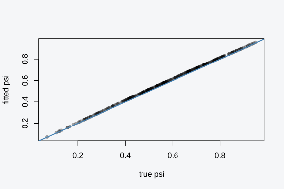

Fitted occupancy probability against the true simulated probability, scattered around the identity line

The same fitted object answers the standard accessors, and they behave the same way on a Laplace fit and a NUTS fit. The Laplace tier reports the Gaussian approximation at the mode; the sampler tier reports empirical posterior summaries from the draws. The call shape stays the same across both.

Accessor	Returns
`coef()`	per-process fixed-effect estimates
`summary()`	estimate, SD, credible bounds (plus Rhat/ESS under NUTS)
`confint()`	credible intervals as a matrix
`vcov()`	fixed-effect covariance
`fitted()`	per-site `psi`, `p`, `z`
`predict()`	occupancy at a new design or varied term
`waic()`	WAIC, elpd, effective parameters
`residuals()`	deviance / Pearson / response residuals
`simulate()`	replicate detection histories from the fit

Checking the fit

A recovered set of coefficients is not the same as a model that describes the data. Recovery in simulation tells you the fitter can find the truth when the truth matches the model; it says nothing about whether your model matches the data in front of you. Three checks ask the second question from different angles: an information criterion for predictive accuracy, a posterior predictive check for whether replicated data look like the real data, and a calibration check on the per-site residuals.

waic() computes the widely applicable information criterion from the pointwise marginal log-likelihood, along with the expected log predictive density and the effective number of parameters. The marginal log-likelihood is the right input here because it has already summed out the latent state, so the score measures how well the model predicts the detection histories you actually saw rather than the unobservable presences. WAIC is an in-sample predictive score, and on its own one number means little; it earns its keep in the comparison below, against another model fit to the same data.

w <- waic(fit)
c(waic = w$estimates["waic", "Estimate"], elpd = w$estimates["elpd_waic", "Estimate"], p_waic = w$estimates["p_waic", "Estimate"])
#>        waic        elpd      p_waic 
#> 1646.075327 -823.037664    3.811516

The three numbers are facets of one calculation. elpd is the expected log pointwise predictive density, the model’s estimated predictive accuracy on new data of the same shape; higher is better. p_waic is the effective number of parameters, estimated from how much the pointwise log-likelihood varies across the posterior rather than counted from the formula, so it captures the flexibility a model actually used. waic itself is -2 * elpd on the deviance scale, which is why lower is better and why it reads on the same scale as an AIC, with the difference that the penalty is the effective parameter count rather than the nominal one.

ppc() runs a posterior predictive check. It simulates detection histories from the fitted parameters, computes a discrepancy statistic (Freeman-Tukey by default) on the replicates and on the observed data, and reports a Bayesian $p$ -value, the fraction of replicates whose statistic exceeds the observed one. A value near 0.5 means the observed data look like a typical draw from the fitted model; values near 0 or 1 flag a misfit.

pp <- ppc(fit, fit.stat = "freeman-tukey")
pp$bayesian.p
#> [1] 0.478

hist(pp$fit.y.rep, breaks = 30, col = "grey85", border = "white",
     main = "", xlab = "Freeman-Tukey statistic (replicated)")
abline(v = mean(pp$fit.y), col = "firebrick", lwd = 2)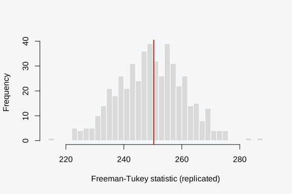

Histogram of replicated Freeman-Tukey statistics with the observed value marked by a vertical line falling inside the bulk

The observed statistic sits inside the bulk of the replicated values, so the fit reproduces the spread of the detection histories. The probability integral transform offers a complementary view. pit_residuals() returns one PIT value per site; under a well-calibrated model they are uniform on $[0, 1]$ , and test_uniformity() runs the formal Kolmogorov-Smirnov test against that target.

pit <- pit_residuals(fit)
hist(pit, breaks = 12, col = "grey85", border = "white",
     main = "", xlab = "PIT residual")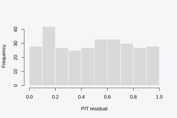

Histogram of PIT residuals across sites, roughly flat between zero and one

test_uniformity(pit)$p.value
#> [1] 0.6501897

The histogram is roughly flat and the test does not reject uniformity, which is the calibration the model promised. The shape of a PIT histogram diagnoses the direction of any miscalibration. A hump in the middle says the model is overdispersed, spreading its predictive mass wider than the data need, so real outcomes land in the centre of their predictive distributions too often. A U-shape says the opposite: the model is overconfident, its intervals too narrow, and real outcomes fall into the tails more than uniformity allows. A flat histogram, as here, says the predictive distribution is the right width.

The per-site residuals give a fourth, more local view. residuals() returns a list with an occupancy component, one residual per site comparing the observed detection indicator against the fitted z, and a detection component at the visit level. Deviance residuals are the default and the natural scale for binary data.

res <- residuals(fit, type = "deviance")
plot(fv$psi, res$occ, pch = 16, col = rgb(0, 0, 0, 0.3),
     xlab = "fitted psi", ylab = "occupancy deviance residual")
abline(h = 0, col = "grey50")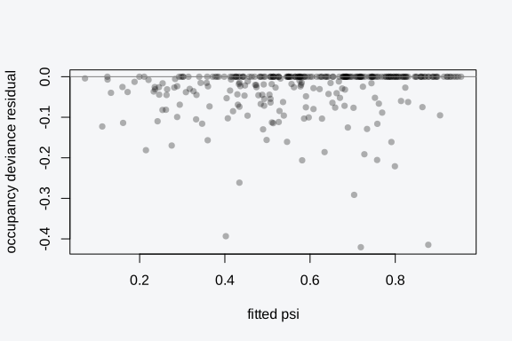

Occupancy deviance residuals against fitted occupancy probability, scattered with no trend

A residual plot with no trend against the fitted values, as here, says the mean structure is adequate; a funnel or a curve would point to a missing covariate or a wrong link. Read all four checks together. WAIC ranks models, the posterior predictive check asks whether the chosen model reproduces the data’s gross features, the PIT asks whether its uncertainty is the right size, and the residuals localise any misfit to particular sites. A model can pass one and fail another, and each failure points somewhere different.

Interpreting the estimates

A fitted occupancy model answers two distinct questions, and the accessors map onto them. One is about the drivers: which covariates move occupancy, which move detection, and by how much. That question is answered by the coefficients and their intervals, read on the logit scale for the sign and significance and on the probability scale for the magnitude. The other is about the sites: where is the species likely to be, accounting for the misses. That question is answered by the fitted z and by prediction at new designs. The two are linked through the same coefficients but ask for different summaries, and confusing them is a common source of misread results.

Start with the drivers. Read the coefficients against their uncertainty rather than as bare points. The occupancy slope on occ_cov1 is positive and its credible interval clears zero, so the covariate is doing real work; the same holds for detection.

ci <- confint(fit)
ci
#>                     2.5 %    97.5 %
#> psi_(Intercept) 0.1095686 0.6181653
#> psi_occ_cov1    0.7082995 1.3154436
#> p_(Intercept)   0.5400064 0.8089798
#> p_det_cov1      0.3724036 0.6451330

The intervals carry the inference. A coefficient whose interval spans zero is not pulling its weight regardless of where the point estimate falls, and the width of the interval tells you how firmly the data pin the effect. The coefficients live on the logit scale, which is where the linear model is additive but not where ecological intuition lives. A slope of 1.0 on occ_cov1 does not mean occupancy rises by one anything; it means the log-odds of occupancy rise by one for each unit of the covariate, and the effect on the probability itself depends on where you start. That is the value of turning a coefficient into a curve on the probability scale.

tobs_marginal_effect() does exactly that. It varies one covariate across the range seen in the data, holds the others at their mean, pushes each draw of the coefficients through the inverse logit, and returns the predicted probability with a 95% credible band. The band is the posterior uncertainty in the curve, narrow where the data are dense and the covariate is near its centre, wider out at the edges. Here it traces how occupancy responds to occ_cov1.

me <- tobs_marginal_effect(fit, "occ_cov1", process = "occupancy")
plot(me)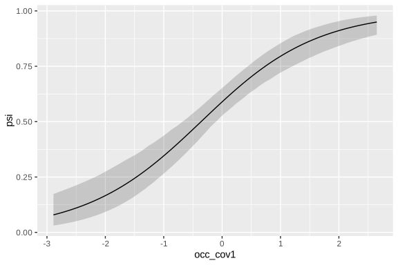

Predicted occupancy probability rising with occ_cov1, with a shaded 95 percent credible band

The curve is the occupancy-covariate relationship on the scale a reader cares about. It rises with occ_cov1, steeply through the middle where the logit is near zero and the probability is most sensitive, and it flattens toward the ends where occupancy approaches its floor and ceiling. The S-shape is the inverse-logit doing its work; a coefficient table hides it, and the plot makes it the headline.

The detection process has its own marginal effect; switch process to read it. The band there reports how sharply detection climbs with det_cov1, and reading it alongside the occupancy curve keeps the two processes distinct in interpretation as well as in the model. A covariate can drive occupancy without touching detection, or the reverse, and plotting each arm separately is how you tell which.

me_det <- tobs_marginal_effect(fit, "det_cov1", process = "detection")
plot(me_det)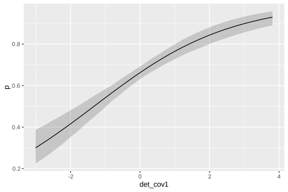

Predicted detection probability rising with det_cov1, with a shaded 95 percent credible band

Prediction

Prediction here means evaluating the fitted occupancy probability at covariate values you choose, with the full posterior uncertainty propagated through. The distinction from the marginal-effect plot is the input: the plot sweeps one covariate across its observed range, while prediction takes an explicit design matrix of the exact rows you want. Use the plot to see a relationship, use prediction to get numbers for specific sites or scenarios, a new reserve at known habitat values, say, or the difference between two management options.

For prediction at an explicit design, pass a matrix to X.0 with one column per occupancy coefficient, the intercept first. The result carries the posterior mean, standard deviation, and credible bounds of $\psi$ at each new row, with the uncertainty drawn from the same fixed-effect covariance the summary reports, so a prediction in a sparsely sampled corner of covariate space comes back with an honestly wide interval.

X0 <- cbind(`(Intercept)` = 1, occ_cov1 = c(-1, 0, 1))
predict(fit, X.0 = X0)
#>        mean         sd      q2.5       q50     q97.5
#> 1 0.3455812 0.04506214 0.2650332 0.3441281 0.4369669
#> 2 0.5893301 0.03180065 0.5267301 0.5882291 0.6518637
#> 3 0.7952724 0.03456338 0.7214816 0.7981468 0.8536645

The columns of X.0 must line up with the occupancy coefficients in order, the intercept first, then each covariate, which is why the example names them. The three rows are a site one standard deviation below the mean, at the mean, and one above. Occupancy climbs from about 0.31 to about 0.79 across that span, with the credible bounds widening at the extremes where the data thin out. This is prediction for the occupancy process alone; the returned $\psi$ is the probability a site at that design is occupied, before any visits. To predict a detection probability instead, the same machinery runs on the detection arm through tobs_marginal_effect(..., process = "detection"). The NUTS fit predicts from its draws rather than a Gaussian approximation, and the two land in the same place when the posterior is well behaved.

predict(fit_nuts, X.0 = X0)
#>        mean         sd      q2.5       q50     q97.5
#> 1 0.3416830 0.04209410 0.2669885 0.3393469 0.4249586
#> 2 0.5917456 0.03045209 0.5338715 0.5928335 0.6539069
#> 3 0.8009468 0.03456605 0.7300807 0.8013661 0.8633308

tobs_marginal_effect() is the right tool for a smooth response curve across one covariate; predict(X.0 = ) is the right tool for the handful of specific designs you actually want a number for.

The uncertainty those predictions carry comes from the fixed-effect covariance, which vcov() exposes directly. The off-diagonal entries record how the estimates move together, and the occupancy intercept and slope are mildly correlated because both are read from the same all-zero sites.

round(vcov(fit), 3)
#>                 psi_(Intercept) psi_occ_cov1 p_(Intercept) p_det_cov1
#> psi_(Intercept)           0.017        0.003         0.000      0.000
#> psi_occ_cov1              0.003        0.024         0.000      0.000
#> p_(Intercept)             0.000        0.000         0.005      0.001
#> p_det_cov1                0.000        0.000         0.001      0.005

simulate() runs the generative process in reverse from a fitted model: it draws new latent states and new detection histories from the posterior, which is the engine behind the posterior predictive check and the dispersion tests above. Calling it directly is useful for a custom check the built-in diagnostics do not cover.

ysim <- simulate(fit, nsim = 1)[[1]]
c(observed_detections = sum(y == 1),
  simulated_detections = sum(ysim == 1))
#>  observed_detections simulated_detections 
#>                  682                  712

The simulated detection count lands near the observed one, as it should when the model fits, since the same parameters generated both up to sampling noise.

Comparing models

WAIC earns its keep in comparison. A single WAIC value is uninterpretable on its own, the way a single likelihood is; what carries meaning is the difference between two models fit to the same data. The criterion estimates out-of-sample predictive accuracy by penalising the in-sample log-likelihood with the effective number of parameters, p_waic, which is read from the variance of the pointwise log-likelihood across the posterior rather than counted by hand. A model that overfits inflates p_waic and pays for it. Fit an intercept-only occupancy model against the covariate model and read the two scores side by side; the lower WAIC is the better predictor of the data you have.

fit0 <- tobs(~ 1, data = dat, family = occu(),
             detection = ~ det_cov1, y = y, method = "laplace",
             control = list(verbose = FALSE))

waic_tab <- data.frame(
  model  = c("intercept only", "with occ_cov1"),
  waic   = c(waic(fit0)$estimates["waic", "Estimate"], waic(fit)$estimates["waic", "Estimate"]),
  p_waic = c(waic(fit0)$estimates["p_waic", "Estimate"], waic(fit)$estimates["p_waic", "Estimate"])
)
waic_tab$delta <- waic_tab$waic - min(waic_tab$waic)
waic_tab
#>            model     waic   p_waic    delta
#> 1 intercept only 1695.349 2.723585 49.27383
#> 2  with occ_cov1 1646.075 3.811516  0.00000

The covariate model carries the lower WAIC, matching how the data were generated: the occupancy slope was 1.0, an effect the intercept-only model has no parameter to represent. The delta column is the gap from the best model. A drop of more than a few units is the usual rough threshold for preferring the larger model, though the comparison is about predictive accuracy and does not certify that either model is correctly specified. WAIC will happily rank two wrong models and hand you the less wrong one. Pair it with the posterior predictive check above before trusting the winner.

The same comparison extends to the detection process. A covariate that belongs in detection but not occupancy, observer experience or survey effort, should lower WAIC when added to the detection formula and barely move it when forced onto the occupancy formula instead. Building the model is partly a matter of deciding which process each covariate enters, and WAIC gives a check on those decisions one covariate at a time. The two extra diagnostics below round out the picture for count-like discrepancies the Freeman-Tukey statistic might miss.

test_dispersion() compares the variance of the per-site detection totals in the data against the variance across simulated replicates, and test_zero_inflation() does the same for the count of all-zero sites. Both return a ratio near one and a $p$ -value near 0.5 when the model reproduces that feature of the data.

disp <- test_dispersion(fit, n.samples = 200)
zi   <- test_zero_inflation(fit, n.samples = 200)
c(dispersion_ratio = disp$ratio, dispersion_p = disp$p.value,
  zero_ratio = zi$ratio, zero_p = zi$p.value)
#> dispersion_ratio     dispersion_p       zero_ratio           zero_p 
#>        0.9901005        0.5550000        1.0024664        0.4950000

A dispersion ratio above one with a small $p$ -value would say the detection totals vary more than the fitted model expects, a sign of unmodelled site heterogeneity that a random effect or an extra covariate might absorb. An excess of zero sites beyond what the model predicts points the same direction. Here both ratios sit near one, so the simple model already accounts for the spread and the zeros in the data.

WAIC also settles the structural question of which process a covariate belongs to. det_cov1 was generated as a detection covariate, so it should lower WAIC when it sits in the detection formula and do little when forced onto the occupancy formula instead. Fit both misallocations against the correct model and compare.

fit_det_only <- tobs(~ occ_cov1, data = dat, family = occu(),
                     detection = ~ 1, y = y, method = "laplace",
                     control = list(verbose = FALSE))
fit_misplaced <- tobs(~ occ_cov1 + det_cov1, data = dat, family = occu(),
                      detection = ~ 1, y = y, method = "laplace",
                      control = list(verbose = FALSE))

c(correct        = waic(fit)$estimates["waic", "Estimate"],
  no_det_cov     = waic(fit_det_only)$estimates["waic", "Estimate"],
  det_on_occ     = waic(fit_misplaced)$estimates["waic", "Estimate"])
#>    correct no_det_cov det_on_occ 
#>   1646.075   1709.588   1711.050

The correct model, with det_cov1 in the detection formula, carries the lowest WAIC. Dropping the detection covariate raises it, and moving that covariate onto the occupancy process raises it too, because the covariate’s signal lives in detection and the occupancy slot cannot use it. This is how WAIC guides model building one decision at a time: each covariate has a process it belongs to, and the criterion tells you when you have put it in the wrong one.

Identifiability and practical guidance

Occupancy and detection trade off against each other along a ridge in the likelihood. The mechanism is the all-zero sites. A site that records no detections contributes $\psi (1-p)^J + (1-\psi)$ to the likelihood, and for a given number of such sites the model can explain them with low occupancy and high detection, or high occupancy and low detection, almost equally well. The two explanations trace a ridge in the $(\psi, p)$ plane, and what pins a point on that ridge is the rate at which detections eventually arrive at the occupied sites. With many visits, an occupied site almost always produces at least one detection, so the share of all-zero sites that are truly empty is well determined and the ridge collapses to a point. With few visits or low detection, occupied sites go silent often enough that the share is ambiguous, the ridge stays flat, and the two processes are weakly separated.

When the ridge is flat, the Laplace mode can drift away from the posterior mean. The reason is geometric: the Laplace fit reports the mode of the posterior and the curvature there, but the mode of a long curved ridge is not where the probability mass sits, and the two diverge as the ridge flattens. The fit does not fail or warn; it returns a clean point estimate that is simply off-centre. This is documented behaviour at small $J$ and low $p$ , the same regime where a glm fit to a half-identified likelihood would wander, and it is the main thing to watch. NUTS does not have this failure mode, because it integrates over the ridge rather than sitting at its mode, which is why the rule of thumb below is to cross-check the two when detection is marginal.

tobs_check_id() screens the model design and flags the usual trouble: very low or very high naive occupancy, too few visits per site, and collinear occupancy covariates. It reads the tobs_model stored on the fitted object.

chk <- tobs_check_id(fit$model)
#> No identifiability issues detected.
chk$identifiable
#> [1] TRUE

A short simulation shows the drift directly. Build a dataset with only two visits and low detection (intercept $-1.5$ , so baseline detection near 0.18), the regime where the two processes are weakly separated, and fit it both ways.

sim_hard <- simulate_occu(
  N = 200, J = 2,
  n.occ.covs = 1, n.det.covs = 1,
  beta.occ = c(0.3, 1.0),
  beta.det = c(-1.5, 0.3),   # baseline detection near 0.18
  seed = 11
)

fit_lap <- tobs(~ occ_cov1, data = sim_hard$data, family = occu(),
                detection = ~ det_cov1, y = sim_hard$y, method = "laplace",
                control = list(verbose = FALSE))
fit_hmc <- tobs(~ occ_cov1, data = sim_hard$data, family = occu(),
                detection = ~ det_cov1, y = sim_hard$y, method = "nuts",
                control = list(n.iter = 1000, n.warmup = 500, seed = 11,
                               verbose = FALSE))

data.frame(
  term    = names(coef(fit_lap)),
  truth   = c(0.3, 1.0, -1.5, 0.3),
  laplace = round(coef(fit_lap), 2),
  nuts    = round(coef(fit_hmc), 2),
  row.names = NULL
)
#>              term truth laplace  nuts
#> 1 psi_(Intercept)   0.3   -0.20  5.69
#> 2    psi_occ_cov1   1.0    0.98  5.83
#> 3   p_(Intercept)  -1.5   -1.13 -1.76
#> 4      p_det_cov1   0.3    0.18  0.17

The Laplace and NUTS estimates separate here in a way they did not at six visits and detection near 0.67. With two visits and detection below 0.2 an occupied site is missed on both visits with probability $(1 - 0.18)^2 \approx 0.67$ , so two of every three occupied sites look exactly like empty ones, and the data carry little to anchor the occupancy intercept. The Laplace mode wanders from the posterior centre the sampler reports, and the disagreement between the two columns is the diagnostic. The fix is more visits, more sites, or trusting the sampler over the mode.

The disagreement is the whole point of fitting both. On real data there is no truth column to check against, so the cross-engine comparison stands in for it: when the deterministic mode and the sampled posterior mean tell the same story, the cheap fit is trustworthy, and when they part ways, the geometry has gone bad and only the sampler is reliable. This is cheaper than it sounds, since the Laplace fit is near-instant and a short NUTS run settles the question in seconds for a few hundred sites. Make the comparison a habit whenever detection looks marginal or the visits are few.

Sites, visits, and what you can estimate

The design is two numbers, the count of sites and the count of visits per site, and they buy different things. Sites buy resolution on occupancy: each site is one draw of the latent state, so the occupancy coefficients sharpen as the site count grows, the same way a logistic regression sharpens with sample size. Visits buy the separation between occupancy and detection: each extra visit to an occupied site is another chance to break an all-zero history, which is what tells true absence apart from missed presence. A study with thousands of sites and one visit each can estimate detection-blind prevalence but cannot correct for detection at all; a study with a handful of sites visited many times each can pin detection but says little about what drives occupancy across the landscape. Most occupancy designs want a balance, many sites with a modest number of visits, and the right split depends on how detectable the species is. A conspicuous species needs few visits per site and can spend its budget on sites; a cryptic one needs more visits before each site’s history is informative, and the same budget buys fewer sites.

A few numeric rules of thumb fall out of this.

Aim for at least three visits per site, more when detection is low. Two visits can identify occupancy and detection in principle, but the ridge is steep and the Laplace mode is fragile. Three to five visits is the comfortable range for moderate detection; push toward six or more when per-visit detection drops below about 0.3, since each visit then carries little signal and you need more of them.
Keep naive occupancy between roughly 0.1 and 0.9. When fewer than about 10% of sites record any detection, the occupancy coefficients are barely informed and the standard errors balloon. Above about 90% there is almost no variation in the latent state for a covariate to explain. tobs_check_id() warns at the 5% and 95% edges.
A few hundred sites is a working minimum for covariate effects. Recovering an occupancy slope to useful precision wants on the order of 200 or more sites; with a few dozen, fit an intercept-only model and report occupancy as a single number rather than chasing covariate effects the data cannot support.
Switch to NUTS when the Laplace and NUTS coefficients disagree. Fit both, as the drift example above does, and compare the coefficient columns. When they agree to within a few percent, the cheap deterministic fit is faithful and you keep it, including for the WAIC comparisons, since the marginal likelihood it scores is the same one the sampler targets. When they pull apart, the posterior is not Gaussian at its mode, the Laplace point estimate is off-centre, and the sampler is the honest answer despite the extra runtime.
Treat all-zero sites as information, not as missing data. The instinct to drop sites with no detections is exactly wrong: those sites are where the occupancy-detection separation lives, and discarding them throws away the signal the model needs. Keep them in y as rows of zeros.

These thresholds are guidance, not hard cutoffs. A study with two visits and high detection can be perfectly identified, and one with six visits and detection near 0.05 can still struggle. The reliable test is the one the drift example demonstrates: fit under both engines and see whether they agree.

When not to reach for a single-season occupancy model at all: if you only ever visited each site once, there is no replication to separate detection from occupancy, and the model is unidentified no matter which engine you run. A single visit per site collapses the two branches of the likelihood into a plain Bernoulli regression on whatever you recorded, with detection and occupancy hopelessly confounded into one fitted probability, and no amount of computation recovers the two underlying processes from data that never observed them separately. The same warning applies, more softly, to designs where almost every site was visited once and only a handful were revisited: the revisited sites carry the entire detection signal, and the model leans on them harder than their number suggests. When the design genuinely lacks replication, the honest moves are to add repeat visits in the next season, to borrow strength from a spatial or random-effect structure that ties sites together so neighbours inform each other’s detection, or to report a raw detection-corrected presence map only where the survey effort actually supports the correction. A model that returns a clean-looking number from data that cannot identify it is worse than no model, because the number invites a confidence the design never earned.

Where to go next

N-mixture abundance, negative binomial, and areal spatial counts: vignette("abundance").
Many species at once with community hyperpriors: vignette("community-models").
Colonisation and extinction across seasons: vignette("dynamic-occupancy").
Random effects with lme4 bar syntax: vignette("random-effects").
Posterior-predictive checks, WAIC, and spatial residual diagnostics in depth: vignette("diagnostics").