Installation
install.packages("pak")
pak::pak("gcol33/tulpaObs")            # latest from GitHub
pak::pak("gcol33/tulpaObs@v0.1.1")     # a specific tagged release
Tagged releases are listed at https://github.com/gcol33/tulpaObs/releases.
pak resolves the dependency tree, pulling tulpa and
tulpaMesh from the r-universe repository DESCRIPTION
declares in Additional_repositories, at or above the
Imports floor. A C++17 toolchain is needed (Rtools on
Windows, Xcode CLI tools on macOS, r-base-dev on Linux);
both tulpa and tulpaObs compile their backends
on first install.
From presence to counts
Occupancy models ask one question per site: is the species there or not. A repeated-count survey asks a harder one. A surveyor visits a site five times and records not whether a marbled salamander was seen, but how many: 3, then 1, then 4, then 0, then 2. Those numbers carry more than presence. They carry the size of the local population, blurred by the fact that nobody counts every individual on every visit.
Royle’s (2004) N-mixture model is the tool for that data. It keeps the two-level structure occupancy taught us, a true state we cannot see and a noisy observation we can, but the latent state is now a count rather than a coin flip. Each site holds some unknown number of animals , fixed across the short survey window. On each visit the surveyor detects each animal independently with probability , so the recorded count is a thinned version of . Five visits to a site with eight animals and detection 0.4 might read 4, 2, 3, 4, 1. The counts never reach eight, and the model’s job is to see eight through the thinning.
This buys you something occupancy cannot give. Where occupancy estimates the probability a site is used, N-mixture estimates how many individuals use it, and how that number responds to a covariate, all from counts that systematically undercount. The price is the same identifiability tension occupancy has, sharpened: abundance and detection both push the counts down or up, and the data have to separate them. A site that averages two animals per visit is consistent with twenty animals seen one in ten times, or with three animals seen two in three times. What breaks the tie is the spread of the counts across visits. Twenty animals at detection 0.1 produce counts that jump around a lot relative to their mean; three animals at detection 0.67 produce counts that barely move. The model reads that spread and infers the abundance behind it. More visits sharpen the read, and counts that vary across them are what carry the information at all.
The model leans on one assumption worth naming up front: the population is closed across the survey window. The animals at a site stay put and stay the same animals from the first visit to the last, so every count is a thinning of the same latent number. A survey spread over a season that lets animals move in and out, breed, or die violates this, and the model will read the movement as detection noise. The closure window is usually a few days to a few weeks, short enough that the standing population is fixed but long enough to gather replicate counts. Designing the survey to respect that window matters as much as any modelling choice that follows.
This vignette builds an N-mixture fit from a simulation with known truth, reads the estimates back, handles the count-ceiling parameter, switches to a negative-binomial state for overdispersed counts, predicts abundance at new covariate values, adds an areal spatial field, and closes with the rules of thumb that decide when the model is the right one.
The model
Write the two levels for site and visit . The latent abundance is Poisson with a log-linear mean, and the counts are binomial thinnings of that abundance with a logit-linear detection:
Here is the expected abundance at site , driven by site covariates through a log link, and is the per-individual detection probability on visit , driven by detection covariates through a logit link. The abundance arm uses a log link because is a rate that must stay positive; that detail comes back the first time you read a coefficient.
The latent never appears in the data. What occupancy did with a single sum over , N-mixture does with a sum over every possible abundance:
The sum runs from the largest count seen at the site (you cannot have fewer animals than you counted on your best visit) up to a ceiling . This marginal has a closed form, so tulpa evaluates it directly with analytical gradients and reads the curvature at the mode for standard errors. There is no EM loop and no data augmentation over : the latent count integrates out exactly, term by term, which is why the fit returns in a fraction of a second. The ceiling is the one approximation, and the next sections treat it as such.
The exact marginalisation is what separates this from occupancy mechanically. An occupancy model sums over two states and the arithmetic is trivial. An N-mixture model sums over a few hundred, and a naive implementation would recompute the binomial product for every candidate at every site on every gradient step. tulpa caches the parts of each term that do not depend on the coefficients, so the repeated evaluations across the optimisation reuse work rather than redo it. The practical effect is that a fit on a few hundred sites with a ceiling in the low hundreds is a sub-second operation, not a sampler you wait on. The same closed form also means the standard errors are the genuine observed-information curvature of the marginal, not a Monte-Carlo approximation, so the credible intervals are deterministic and repeatable across runs.
One consequence of the log link deserves a flag before the first fit.
A coefficient on the abundance arm is a multiplicative effect on
expected abundance, not an additive one. A slope of 0.5 means a one-unit
increase in the covariate multiplies
by
,
a 65 percent rise, and the same slope adds more animals where abundance
is already high than where it is low. The intercept is the log of
baseline abundance, so it reads as a number of animals only after
exp(). This is the same arithmetic a Poisson GLM uses, and
the coefficients carry the same interpretation; the only twist is that
the counts feeding them are thinned, and the model corrects for the
thinning before it reports the slope.
Simulating and fitting a Poisson model
simulate_abun() draws a dataset with the truth you set,
so the fit has a target to recover. Abundance depends on one site
covariate with intercept
(so baseline expected abundance is 3 animals) and slope 0.5; detection
depends on one covariate with intercept 0.4 (detection near 0.6) and
slope 0.3. Five visits per site give the thinning enough replication to
separate the two arms.
sa <- simulate_abun(
  N = 200, J = 5,
  n.abund.covs = 1, n.det.covs = 1,
  beta.lambda = c(log(3), 0.5),   # log link: intercept is log(baseline lambda)
  beta.p      = c(0.4, 0.3),      # logit link on detection
  seed = 2
)
dat <- sa$data       # site covariates, one row per site
y   <- sa$y          # 200 x 5 count matrix
y[1:4, ]
#>      [,1] [,2] [,3] [,4] [,5]
#> [1,]    1    1    0    1    1
#> [2,]    3    2    0    1    2
#> [3,]    0    1    1    1    0
#> [4,]    1    1    1    0    1
The counts undercount the latent abundance. Averaging the per-site maximum count against the simulated truth shows the gap that detection opens.
c(mean_max_count = mean(apply(y, 1, max)),
  mean_true_N    = mean(sa$truth$N))
#> mean_max_count    mean_true_N
#>          2.820          3.275
The fit follows the same call shape as occupancy. The abundance
formula is the first argument, detection is its own formula, and
abun() selects the N-mixture family.
method = "laplace" is the default; it finds the mode of the
marginal likelihood and the curvature there. A shared areal field fits
under method = "nested_laplace" (used in the spatial
section below), and method = "nuts" samples the closed-form
marginal in full when you want the whole posterior rather than the
Laplace approximation.
fa <- tobs(
  ~ abund_cov1,
  data      = dat,
  family    = abun(),
  detection = ~ det_cov1,
  y         = y,
  method    = "laplace",
  control   = list(verbose = FALSE)   # the fitter prints iterations otherwise
)
coef() returns the estimates named by arm
(lambda_, p_). Read the lambda
arm with the log link in mind: the intercept is on the log scale, so
back-transforming with exp() gives baseline expected
abundance.
coef(fa)
#> lambda_(Intercept)  lambda_abund_cov1      p_(Intercept)         p_det_cov1
#>          1.0671676          0.4453561          0.4086084          0.2462074
c(baseline_lambda = exp(coef(fa, arm = "lambda")[["(Intercept)"]]),
  true_baseline   = 3)
#> baseline_lambda   true_baseline
#>        2.907134        3.000000
The abundance intercept back-transforms to roughly the three animals
the data were built with, and the slope on abund_cov1 lands
near the simulated 0.5. summary() adds the posterior
standard deviation and the credible bounds for every coefficient; the
lambda_ rows are the abundance arm and the p_
rows the detection arm.
summary(fa)
#>                     estimate  std.error     2.5 %    97.5 %
#> lambda_(Intercept) 1.0671676 0.04902181 0.9747811 1.1612617
#> lambda_abund_cov1  0.4453561 0.03999136 0.3667358 0.5213671
#> p_(Intercept)      0.4086084 0.07297071 0.2728524 0.5536938
#> p_det_cov1         0.2462074 0.06268696 0.1242706 0.3717937
fitted() returns the per-site quantities the fit
implies: expected abundance lambda, detection probability
p, and the posterior mean abundance N given
the counts. The last one is the estimate that matters for a population
total, since it conditions on what was actually seen at each site.
fv <- fitted(fa)
str(lapply(fv, head, 4))
#> List of 3
#>  $ lambda: num [1:4] 1.95 3.15 5.87 1.76
#>  $ p     : num [1:4] 0.618 0.618 0.618 0.618
#>  $ N     : num [1:4] 1.12 3.31 1.02 1.11
Plotting the posterior mean abundance against the simulated truth shows the model recovers the site-level signal through the thinning, not just the population average.
plot(sa$truth$N, fv$N, pch = 16, col = rgb(0, 0, 0, 0.35),
     xlab = "true N", ylab = "fitted E[N | y]")
abline(0, 1, col = "steelblue", lwd = 2)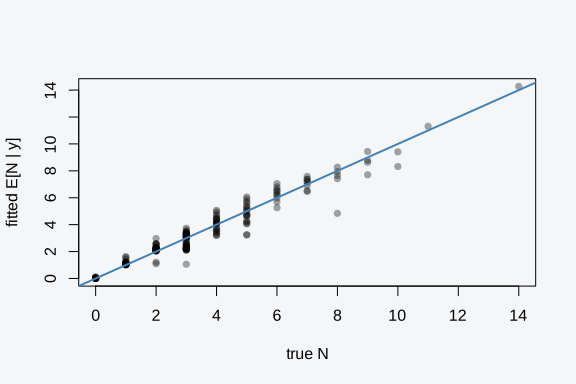
The points track the identity line with scatter that grows at higher abundance, which is the right behaviour: a site with more animals leaves more room for the binomial thinning to vary the counts, so its posterior abundance is less certain.
The count ceiling K.max
The marginal likelihood sums over abundance from each site’s maximum
count up to a ceiling. That ceiling is K.max, and the fit
chooses a default from the data when you do not set it. The sum has to
reach high enough that the Poisson mass above K.max is
negligible; if K.max sits too close to the true abundance,
the model truncates probability that belongs in the likelihood and
biases
downward.
The default works for ordinary counts. You raise K.max
when abundance is large relative to detection, so the latent
can sit far above any single count. A site with
and detection 0.2 might never record more than a dozen animals on a
visit, yet its abundance routinely exceeds thirty, and the sum has to
climb past that. The symptom of a ceiling set too low is a boundary
warning or an abundance estimate that drifts when you raise it. The
check is to refit with a higher K.max and confirm the
estimate is stable.
fa_k <- tobs(~ abund_cov1, data = dat, family = abun(K.max = 200),
             detection = ~ det_cov1, y = y, method = "laplace",
             control = list(verbose = FALSE))
rbind(default_K = coef(fa, arm = "lambda"),
      K_max_200 = coef(fa_k, arm = "lambda"))
#>           (Intercept) abund_cov1
#> default_K    1.067168  0.4453561
#> K_max_200    1.065566  0.4400979
The two fits agree to several decimals, so the default ceiling was
already high enough here. On data where they disagree, take the
higher-K.max fit and keep raising it until the estimate
settles. The cost of a generous ceiling is compute time, since the inner
sum runs over more terms, and that cost is linear in K.max,
so a ceiling a few times the largest plausible abundance is a safe
default rather than an expensive one.
It helps to see why a low ceiling pulls the estimate down. The
likelihood asks how probable the observed counts are under a given
,
and it answers by summing over every abundance that could have produced
them. If the true
wants to place real probability on abundances above the ceiling, cutting
the sum off there throws that probability away. The optimiser then finds
a smaller
that fits its mass entirely below the ceiling, and the abundance
estimate comes out biased low. The bias is invisible in any single fit;
it shows only when you raise the ceiling and watch the estimate move.
That is why the stability check is the diagnostic rather than any one
number. A practical starting point is to set K.max to
several times the largest count you would believe at the most abundant
site, then confirm a doubling of it leaves the coefficients unchanged.
The negative-binomial state, with its heavier tail, needs more headroom
than Poisson for the same mean, so a ceiling that suffices under Poisson
can be tight under overdispersion.
Overdispersion and the negative binomial
The Poisson state assumes the variance of abundance equals its mean. Real populations rarely oblige. Animals cluster, habitat varies in ways no covariate captures, and the spread of true abundance across sites runs wider than Poisson allows. When it does, a Poisson N-mixture absorbs the extra spread into and detection, and the standard errors come out too small.
The biology behind overdispersion is worth holding in mind, because it tells you when to expect it. A Poisson abundance is what you get when individuals settle independently and at the same rate everywhere a covariate says they should. Real animals do neither. They aggregate around resources, they respond to gradients no survey measured, and a good patch holds far more than its covariates predict while a poor one holds far fewer. Each of those produces sites that are more variable than their fitted mean, which is overdispersion exactly. The clustering need not be spatial; it can be any unmeasured driver that makes some sites richer and others poorer than the covariates explain. Whenever you suspect such a driver, and in count data you usually should, the negative binomial is the safer default state.
abun(mixture = "negbin") replaces the Poisson state with
a negative binomial,
,
where the size
sets the overdispersion through
. A small
means heavy clustering; as
grows the negative binomial approaches the Poisson, and the extra
parameter costs nothing. Simulate overdispersed counts with
,
so a site with mean abundance 4 has variance
,
three times the Poisson value.
sb <- simulate_abun(
  N = 200, J = 5, n.abund.covs = 1, n.det.covs = 1,
  mixture = "negbin", size = 2,
  beta.lambda = c(log(4), 0.4), beta.p = c(0.5, 0.2),
  seed = 5
)
Fit the negative-binomial model by passing the same
mixture flag to the family. The size
is estimated jointly with the coefficients on the log scale and reported
on the object.
fb <- tobs(~ abund_cov1, data = sb$data, family = abun(mixture = "negbin"),
           detection = ~ det_cov1, y = sb$y, method = "laplace",
           control = list(verbose = FALSE))
coef(fb)
#> lambda_(Intercept)  lambda_abund_cov1      p_(Intercept)         p_det_cov1
#>          1.3186647          0.4671972          0.4868058          0.1193980
#>              log_r
#>          0.9198933
The dispersion lives in fb$nmix_dispersion: the
natural-scale size $r, its log-scale value
$log_r, and the delta-method standard error
$r_sd.
fb$nmix_dispersion
#> $r
#> [1] 2.522005
#>
#> $log_r
#> [1] 0.9250543
#>
#> $r_sd
#> [1] 0.4615203
The estimated sits near the simulated 2, with a standard error wide enough to tell you the size is the least certain quantity in the fit. That is normal. The size is identified only through the tail of the count distribution, and a single dataset of 200 sites pins it loosely.
Fitting a negative binomial when the data are actually Poisson is close to free, since the size simply drifts large. Fitting a Poisson when the data are overdispersed is the costly mistake, because the missing variance has nowhere to go but the standard errors. A quick dispersion check tells you which regime you are in. Compare the variance of the per-site maximum count against its mean: a ratio well above one is the signature of overdispersion that a Poisson state cannot represent.
maxcount <- apply(sb$y, 1, max)
c(mean = mean(maxcount), var = var(maxcount),
  ratio = var(maxcount) / mean(maxcount))
#>     mean      var    ratio
#> 3.510000 9.306432 2.651405
A ratio near one says Poisson will do; a ratio of two or more says reach for the negative binomial. This is a rough diagnostic on the observed counts, not the latent state, so treat it as a flag rather than a test. The cleaner comparison is to fit both and read the marginal log-likelihood, which the next-to-last section does.
Predicting abundance
predict() with a design matrix X.0 returns
the abundance arm’s prediction at new covariate values, on the response
scale, with the posterior spread propagated through the joint
coefficient covariance. Pass one column per abundance coefficient.
X0 <- cbind(`(Intercept)` = 1, abund_cov1 = c(-1.5, 0, 1.5))
predict(fa, X.0 = X0)
#>       mean        sd     q2.5      q50    q97.5
#> 1 1.496578 0.1350134 1.248987 1.483833 1.776139
#> 2 2.910627 0.1428580 2.650587 2.909445 3.193961
#> 3 5.681138 0.3554934 5.033413 5.672292 6.400644
Expected abundance climbs across the three covariate values, and the
credible bounds widen with the mean, the multiplicative spread a log
link produces. That widening is what the log link means. A fixed
uncertainty on the log scale becomes a proportional uncertainty on the
count scale, so a prediction of 8 animals carries a wider absolute band
than a prediction of 2, even when the coefficient is equally well known.
Reading the bounds on the response scale, as predict()
returns them, keeps that proportionality visible rather than hiding it
on the log scale where it looks constant.
The draws behind these summaries come from the joint coefficient
covariance, so the abundance and detection arms vary together rather
than independently. This matters for any quantity that combines the two,
a detection-corrected total or a ratio of abundances at two covariate
values, because the two arms are negatively correlated through the
counts: a fit that nudges detection up has to nudge abundance down to
match the same counts. Drawing them jointly propagates that correlation
into the derived quantity, where drawing them separately would overstate
its uncertainty. To trace the response across the whole covariate range
rather than at three points, pass terms and the predictor
name; the result carries an estimate and a band at each grid point,
ready to plot.
pr <- predict(fa, terms = "abund_cov1")
plot(pr$x, pr$estimate, type = "n",
     xlab = "abund_cov1", ylab = "expected abundance",
     ylim = range(pr$lower, pr$upper))
polygon(c(pr$x, rev(pr$x)), c(pr$lower, rev(pr$upper)),
        col = adjustcolor("steelblue", 0.25), border = NA)
lines(pr$x, pr$estimate, lwd = 2)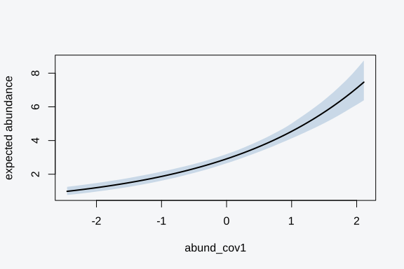
The band is the abundance arm’s uncertainty alone. The detection arm
has its own prediction surface, reached with
type = "detection", which is the right call when the
question is about survey efficiency rather than population size.
Random effects on abundance
Counts arrive grouped. Sites cluster into watersheds, plots nest inside forest stands, transects fall under the field crew that walked them. The group carries its own baseline abundance that no measured covariate captures, and treating that grouping as one fixed intercept per level burns a parameter on every group and leaves the sparse ones with wild estimates. A random intercept ties the levels together instead: each group’s abundance baseline is a draw from , and the model estimates the single spread rather than one free intercept per group. Groups with many sites keep their own signal; groups with few are pulled toward the population mean, the shrinkage that is the point of the random effect rather than a side effect of it.
abun() carries the lme4 bar syntax on
either arm. A term in the abundance formula varies log-abundance by
group; a term in the detection formula varies the logit of
detection. The single-species N-mixture takes (1 | g) for a
random intercept and the slope variants (x | g),
(x || g), and (1 + x | g) the same way the
occupancy model does, with one restriction: a term cannot sit on both
arms of one fit, and a random effect cannot share a fit with an areal
spatial field. Either of those needs the joint sampler. Put the bar on
one arm at a time and the deterministic path handles it.
Simulate grouped abundance with eight watersheds, each holding its
own log-abundance offset drawn from
,
on top of a site covariate x1. Detection is constant near
0.5, and four visits give the thinning enough replication.
sim_re <- function(N = 120, J = 4, ngrp = 8, sigma_b = 0.6, seed = 11) {
  set.seed(seed)
  grp <- rep(seq_len(ngrp), length.out = N)
  b   <- rnorm(ngrp, sd = sigma_b)
  dat <- data.frame(x1 = rnorm(N), g = factor(grp))
  eta <- as.numeric(model.matrix(~ x1, dat) %*% c(0.6, 0.4)) + b[grp]
  Nlat <- rpois(N, exp(eta))
  y <- matrix(NA_integer_, N, J)
  for (i in seq_len(N)) y[i, ] <- rbinom(J, Nlat[i], plogis(0))
  list(y = y, data = dat, b = b)
}
sr <- sim_re()
The fit reads like the others, with the bar inside the abundance
formula. control = list(n.quad = 5) sets the adaptive
Gauss-Hermite resolution that debiases the small-cluster variance
attenuation; n.quad = 1 is the plain joint Laplace, and
higher values recover the spread the single Gaussian per group
misses.
fr <- tobs(
  ~ x1 + (1 | g),
  data      = sr$data,
  family    = abun(),
  detection = ~ 1,
  y         = sr$y,
  method    = "laplace",
  control   = list(n.quad = 5, verbose = FALSE)
)
coef(fr, arm = "lambda")
#> (Intercept)          x1
#>   0.4106965   0.5210838
The abundance intercept and slope recover near the simulated 0.6 and
0.4 with the group structure absorbed into the random effect rather than
blended into the coefficients. The variance component lives in
fr$means under a sigma_g-prefixed name, the
spread across watershed baselines.
sig_name <- grep("^sigma_g", names(fr$means), value = TRUE)
c(estimate = fr$means[[sig_name]], truth = 0.6)
#>  estimate     truth
#> 0.7453534 0.6000000
vcov() returns the joint fixed-effect covariance over
the abundance and detection coefficients alone, the same block the
non-grouped fit carries. The variance-component point estimate sits
outside it, since the marginal-Hessian path does not surface its joint
posterior covariance with the fixed effects.
round(vcov(fr), 4)
#>                    lambda_(Intercept) lambda_x1 p_(Intercept)
#> lambda_(Intercept)             0.0838   -0.0024       -0.0068
#> lambda_x1                     -0.0024    0.0055       -0.0006
#> p_(Intercept)                 -0.0068   -0.0006        0.0199
ranef() returns the per-group effects, the BLUPs, one
row per group level and coefficient: the arm, the grouping factor, the
level, the term, the estimate, and its standard error. The standard
error is the genuine AGHQ marginal posterior spread, wider for groups
with fewer sites.
re <- ranef(fr)
re
#>      arm group level        term    estimate std.error
#> 1 lambda     g     1 (Intercept) -0.05460644 0.2092936
#> 2 lambda     g     2 (Intercept)  0.03921651 0.2190470
#> 3 lambda     g     3 (Intercept) -1.08035897 0.3048384
#> 4 lambda     g     4 (Intercept) -0.44822134 0.2898862
#> 5 lambda     g     5 (Intercept)  0.72807203 0.1509854
#> 6 lambda     g     6 (Intercept) -0.70742394 0.2566427
#> 7 lambda     g     7 (Intercept)  1.02900226 0.1385809
#> 8 lambda     g     8 (Intercept)  0.68121607 0.1538180
Plot the recovered group effects against the simulated truth with the BLUP standard error as an interval. The points track the identity line, with the shrinkage that pulls sparse groups toward zero and the uncertainty band that widens where a group carries less data.
library(ggplot2)
re$truth <- sr$b[as.integer(re$level)]
ggplot(re, aes(truth, estimate)) +
  geom_abline(slope = 1, intercept = 0, colour = "steelblue", linewidth = 1) +
  geom_errorbar(aes(ymin = estimate - std.error, ymax = estimate + std.error),
                width = 0, colour = "grey50") +
  geom_point(size = 2) +
  labs(x = "true group effect", y = "estimated BLUP") +
  theme(panel.background = element_rect(fill = "transparent"),
        plot.background  = element_rect(fill = "transparent"))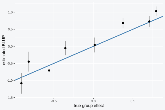
The same machinery moves to detection by writing the bar in the
detection formula, where it varies the per-group logit of
detection and the variance component is named sigma_p for
the detection arm. Under mixture = "negbin" the random
effect and the overdispersion size are estimated together on the same
AGHQ likelihood, with the size as the trailing log-scale coordinate. The
recovery here used eight groups; the variance starts to mean something
around five to eight levels, and below that a fixed effect that names
each group is the honest choice.
Counts on a map
Sites near each other often hold similar numbers of animals for reasons no covariate records: shared microclimate, a corridor of good habitat, a patch the survey design happened to cluster. Left unmodelled, that structure does two kinds of damage. It inflates confidence in the slopes, because neighbouring sites carry correlated leftovers and the model counts each as fresh information when they are partly the same observation seen twice. And it biases the slopes themselves whenever a covariate is spatially patterned, since the covariate and the unmeasured regional driver vary together and a model with nowhere to put the driver loads it onto the covariate. An areal spatial field gives the regional signal a place to live, one random effect per spatial unit, tied to neighbours so the surface stays smooth. The slope is then read against a background that already accounts for location, and its standard error widens to its honest size because the field, not the covariate, now carries the autocorrelation.
The same logic that motivates a spatial field for a binomial or Gaussian response carries over to counts unchanged. What differs is only where the field attaches: it enters the log-abundance predictor, alongside the covariate slopes, so it soaks up the regional variation in how many animals a site holds. The detection arm is left non-spatial here, which is the usual choice, since detection is a property of the survey rather than the place. If survey effort is itself spatially clustered, a field on detection is possible too, but the common case puts the field on abundance and reads it as the smoothed map of population density the covariates do not explain.
For N-mixture the field attaches to the abundance arm through a
spatial term inside the formula, with
method = "nested_laplace". The areal terms are
icar(), bym2(), and car_proper();
each takes a dense 0/1 adjacency matrix with one row and column per
site. Build a small grid and its rook adjacency, where each cell
neighbours the cells directly above, below, left, and right.
grid_adj <- function(side) {
  ng <- side * side
  co <- expand.grid(x = seq_len(side), y = seq_len(side))
  adj <- matrix(0L, ng, ng)
  for (i in seq_len(ng)) for (j in seq_len(ng)) {
    if (i != j && abs(co$x[i] - co$x[j]) + abs(co$y[i] - co$y[j]) == 1L)
      adj[i, j] <- 1L
  }
  adj
}
adj <- grid_adj(6)        # 36 cells, one site per cell
dim(adj)
#> [1] 36 36
Simulate counts on the grid with a smooth abundance field added to the log-linear mean, then thin them to visits. The field is the regional signal the fit has to recover alongside the covariate slope.
sim_spatial <- function(adj, b_lambda, b_p, J = 5, sd_phi = 0.6, seed = NULL) {
  if (!is.null(seed)) set.seed(seed)
  ng <- nrow(adj)
  phi <- as.numeric(scale(rnorm(ng)))
  for (rep in 1:3) {                       # smooth toward neighbours
    pn <- phi
    for (i in seq_len(ng)) {
      nb <- which(adj[i, ] == 1L)
      pn[i] <- 0.5 * phi[i] + 0.5 * mean(phi[nb])
    }
    phi <- pn
  }
  phi <- sd_phi * as.numeric(scale(phi)); phi <- phi - mean(phi)
  x_ab <- rnorm(ng); x_det <- rnorm(ng)
  lambda <- exp(b_lambda[1] + b_lambda[2] * x_ab + phi)
  p <- plogis(b_p[1] + b_p[2] * x_det)
  N <- rpois(ng, lambda)
  y <- matrix(NA_integer_, ng, J)
  for (i in seq_len(ng)) y[i, ] <- rbinom(J, N[i], p[i])
  list(y = y, data = data.frame(abund_cov1 = x_ab, det_cov1 = x_det),
       phi = phi)
}
ss <- sim_spatial(adj, b_lambda = c(log(5), 0.5), b_p = c(0.3, 0.4), seed = 42)
Fit the spatial model with a bym2() term on the
abundance formula. The field’s smoothing strength is integrated over a
grid rather than fixed, so the slope standard errors carry the field’s
own uncertainty. The fit returns the same tobs_fit object
as the non-spatial path, with fs$method reading
"nested_laplace".
fs <- suppressWarnings(tobs(
  ~ abund_cov1 + bym2(graph = adj),
  data      = ss$data,
  family    = abun(),
  detection = ~ det_cov1,
  y         = ss$y,
  method    = "nested_laplace",
  control   = list(verbose = FALSE, max.iter = 50)
))
coef(fs)
#> lambda_(Intercept)  lambda_abund_cov1      p_(Intercept)         p_det_cov1
#>         1.64698503         0.46238494        -0.03558411         0.32983111
The covariate slopes recover with the regional signal absorbed into
the field rather than blended into the coefficient:
coef(fs) reads back the abundance slope near the simulated
0.5 and the detection slope near 0.4.
Read the slopes, not the abundance intercept, under an intrinsic
field. The intrinsic prior pins the field only up to an overall level,
so the intercept and the field mean trade off along a flat direction;
the BYM2 field’s independent component tames that confounding but the
slopes are the inferential payload regardless. The recovered field comes
back on the object as fs$spatial_field, one value per cell,
and cor(fs$spatial_field, ss$phi) is positive: the fit
cannot reconstruct one draw of a noisy field exactly, but it recovers
its shape, and that shape is what removes the bias from the slopes.
c(field_cor = cor(fs$spatial_field, ss$phi),
  method    = fs$method)
#>           field_cor              method
#> "0.906389733746009"    "nested_laplace"
Under mixture = "negbin" the size
is integrated over the outer grid alongside the field’s smoothing
parameters and reported in fs$nmix_hyper$r rather than as a
coefficient, so the spatial path handles overdispersion without adding a
fixed parameter to the covariance.
Comparing models and practical guidance
Does the negative binomial earn its extra parameter? Fit both states
on the overdispersed data and read the marginal log-likelihood through
logLik(). The marginal already integrates the latent
abundance out, so a higher value means the state genuinely fits the
counts better, not that it has more freedom.
fb_pois <- tobs(~ abund_cov1, data = sb$data, family = abun(),
                detection = ~ det_cov1, y = sb$y, method = "laplace",
                control = list(verbose = FALSE))

c(poisson = as.numeric(logLik(fb_pois)),
  negbin  = as.numeric(logLik(fb)))
#>   poisson    negbin
#> -1526.102 -1476.182
The negative binomial carries the higher log-likelihood on data built with , which is the answer the simulation should give. On real data the same comparison decides the state: a meaningfully higher negative-binomial log-likelihood says the counts are overdispersed and the Poisson was hiding it in the standard errors. A near-tie says Poisson is adequate and the simpler state is the honest choice.
A handful of rules of thumb make the rest of the modelling decisions.
At least three visits, more when detection is low. The abundance and detection arms separate only through the spread of counts across visits. With two visits and detection below about 0.3 they are weakly identified, and the abundance estimate can drift toward the count ceiling or collapse toward the mean count. Three visits is the practical floor; five or more is comfortable, and they buy more than extra sites do because replication, not site count, is what pins detection.
Counts must vary within a site. A site that reads 2, 2, 2, 2 tells the model almost nothing about detection, since constant counts are consistent with high abundance and high detection or low abundance seen perfectly. Variation across visits is the signal the binomial thinning leaves, and it is what the detection arm reads. If your counts barely move across visits, the fit will lean on the prior and the covariates rather than the data.
Check the dispersion before trusting Poisson standard errors. A variance-to-mean ratio of the per-site counts above roughly two is a flag for the negative binomial. Fitting Poisson on overdispersed counts does not bias the slopes badly, but it understates their uncertainty, so a coefficient can read significant when it is not. When in doubt, fit both and compare the marginal log-likelihood.
Raise K.max when abundance dwarfs detection. The default ceiling suits ordinary counts. When expected abundance is large and detection is small, the latent sits far above any visit’s count, and a ceiling set too low truncates the likelihood and biases down. A workable rule is to set
K.maxto roughly three to five times the largest count you would believe at the richest site, then double it and confirm the coefficients do not move. The negative-binomial state needs the upper end of that range for the same mean, since its heavier tail puts mass higher.Group with five to eight levels before trusting the variance. A random effect on the abundance arm estimates the spread across groups, and with two or three groups there is almost no information about that spread. Five to eight levels is the rough floor; below it, name each group with a fixed intercept instead. Keep at least ten sites per group when the term carries a random slope rather than only an intercept, since a slope asks each group’s own data to inform its covariate effect before shrinkage.
When N-mixture is the wrong tool. Three cases call for a different model. If the surveys are not closed, animals moving in and out between visits so abundance is not fixed, the binomial thinning assumption breaks and the model reads movement as detection. If you only have detection or non-detection rather than counts, occupancy is the honest model and N-mixture adds a latent abundance the data cannot inform. And if detection is near one, the counts are nearly the abundance itself, so a plain Poisson or negative-binomial regression on the counts is simpler and loses nothing.
Where to go next
- Single-season occupancy, the binary cousin of this model, with the
same detection structure:
vignette("occupancy"). - Many species at once, each with its own N-mixture, tied by community
hyperpriors:
vignette("community-models"). - Grouped random effects in full, with slopes, the
||forms, and the AGHQ debias:vignette("random-effects"). - Areal and continuous spatial fields in depth, with field extraction
and the smoothing-precision posterior: the
tulpaspatial vignettes. - Posterior-predictive checks and residual diagnostics:
vignette("diagnostics").