Diagnostics: checking, comparing, and residuals • tulpaObs

Installation

install.packages("pak")
pak::pak("gcol33/tulpaObs")            # latest from GitHub
pak::pak("gcol33/tulpaObs@v0.1.1")     # a specific tagged release

Tagged releases are listed at https://github.com/gcol33/tulpaObs/releases.

pak resolves the dependency tree, pulling tulpa and tulpaMesh from the r-universe repository DESCRIPTION declares in Additional_repositories, at or above the Imports floor. A C++17 toolchain is needed (Rtools on Windows, Xcode CLI tools on macOS, r-base-dev on Linux); both tulpa and tulpaObs compile their backends on first install.

library(tulpaObs)

A fit to check

A coefficient table tells you what the model thinks. It does not tell you whether the model is any good. This vignette covers the second question: once tobs() returns a fit, how do you decide whether to trust it, how do you choose between two candidates, and where do you look when something is off. The tools split into three groups. WAIC ranks models against each other. Posterior-predictive checks and the simulation-based tests ask whether the fit reproduces features of the data it saw. Residuals localise the trouble to particular sites or visits.

The three groups answer different questions, and confusing them is the most common mistake. Model comparison is relative: it picks the best of the candidates you supply and says nothing about whether the winner is right in any absolute sense. Goodness-of-fit checks are absolute, or aim to be: they compare the fit against the data directly, with no rival model in the frame. Residual analysis is diagnostic: it does not return a verdict but points at the sites and visits driving any misfit the other two flagged. A thorough check uses all three, in that order, because a model can win a comparison, fail a goodness-of-fit check, and have the failure traced to a handful of sites by its residuals.

Occupancy adds a wrinkle that single-process models do not have. The data you observe are detections, but the quantity of interest is occupancy, and the link between them runs through a latent state you never see directly. The posterior-predictive check and the PIT residuals both handle this by conditioning on the latent state given the detection history, rather than redrawing it from the fitted occupancy probability.

Everything below runs on one occupancy dataset, so the diagnostics stay comparable. simulate_occu() gives us a model with known truth: occupancy rises with occ_cov1 (intercept 0.3, slope 1.0), detection depends on det_cov1 (intercept 0.7, so detection near 0.67), and six visits per site keep the two processes apart.

sim <- simulate_occu(
  N = 300, J = 6,
  n.occ.covs = 1, n.det.covs = 1,
  beta.occ = c(0.3, 1.0),
  beta.det = c(0.7, 0.6),
  seed = 1
)
dat <- sim$data
y   <- sim$y

Fit the model the data were generated from. The Laplace engine is the default; verbose = FALSE keeps the EM from printing its iterations.

fit <- tobs(
  ~ occ_cov1,
  data      = dat,
  family    = occu(),
  detection = ~ det_cov1,
  y         = y,
  method    = "laplace",
  control   = list(verbose = FALSE)
)
coef(fit)
#> psi_(Intercept)    psi_occ_cov1   p_(Intercept)      p_det_cov1 
#>       0.3638670       1.0118715       0.6744931       0.5087683

The coefficients land near the truth. That is a good start and nothing more. A model can recover its parameters and still fit badly somewhere the point estimates do not reveal: it might miss a cluster of unusual sites, underpredict the spread of detections, or leave spatial structure in its errors, none of which a coefficient table shows. The job of the diagnostics below is to surface exactly those failures, on a fit whose coefficients already look right, so that the checks are doing real work rather than confirming an obviously broken model.

The one-call panel

Before working through the diagnostics one at a time, check_model() runs the main ones in a single call and prints a compact report. It is the fast first pass: fit the model, call check_model(), and read the headline numbers to decide whether anything needs a closer look. The detailed sections below are where you go once the panel flags something or once you want the plot behind a number.

check_model(fit)
#> === tobs Model Diagnostics ===
#> 
#> Fit: laplace, 1000 posterior draws (no NUTS sampler diagnostics)
#> 
#> WAIC: 1646.1 (p_waic = 3.8)
#> DIC:  1646.3 (p_DIC = 4.0)
#> LPML: -823.1 (elpd_loo = -823.1)
#> 
#> PPC: Bayesian p = 0.488
#> 
#> Zero-inflation: obs=126, exp=126.5, p=0.508
#> Dispersion:     ratio=1.00, p=0.556
#> PIT uniformity: KS D=0.028, p=0.974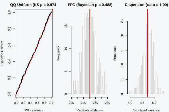

Three diagnostic panels: a QQ plot of PIT residuals against the uniform, a histogram of replicate fit statistics with the observed value marked, and a histogram of simulated variances with the observed variance marked

The report has four blocks, each a condensed form of a section that follows, and the panel beneath it draws the three that have a plot behind them (plot = FALSE prints the report alone). The first line records how the fit was produced. Under method = "laplace" there is no Markov chain, so it reports the draw count and notes that the NUTS sampler diagnostics (divergences, accept probability) do not apply; a fit produced with method = "nuts" prints those instead. The WAIC line is the single number from waic(), useful only against a rival model, with the effective parameter count p_waic alongside. The PPC line is the Bayesian p-value from ppc(); the panel attaches a WARNING: poor fit when it falls below 0.05 or above 0.95, the two-sided cue that the fit fails to reproduce the data. The zero-inflation line reports the observed and expected counts of all-zero sites from test_zero_inflation(). Passing a coords matrix adds a Moran’s I line that warns when residual spatial autocorrelation is significant.

out <- check_model(fit, coords = cbind(dat$occ_cov1, dat$det_cov1))
#> === tobs Model Diagnostics ===
#> 
#> Fit: laplace, 1000 posterior draws (no NUTS sampler diagnostics)
#> 
#> WAIC: 1646.1 (p_waic = 3.8)
#> DIC:  1646.3 (p_DIC = 4.0)
#> LPML: -823.1 (elpd_loo = -823.1)
#> 
#> PPC: Bayesian p = 0.484
#> 
#> Zero-inflation: obs=126, exp=126.9, p=0.552
#> Dispersion:     ratio=1.00, p=0.540
#> PIT uniformity: KS D=0.042, p=0.658
#> 
#> Moran's I: 0.024 (p = 0.000)
#>   WARNING: spatial autocorrelation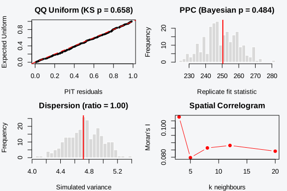

The same diagnostic panels with a fourth added: Moran's I of the occupancy residuals against the number of neighbours

names(out)
#> [1] "waic"           "dic"            "cpo"            "ppc"           
#> [5] "zero_inflation" "dispersion"     "pit"            "uniformity"    
#> [9] "moran"

The panel returns its components invisibly, so out$waic, out$ppc, and out$zero_inflation carry the same objects the individual functions return, ready to feed a table or a plot. The coordinates here are covariate columns standing in for real geography, which is enough to exercise the Moran’s I line; with true site coordinates this is the one call that screens for a missing spatial field at the same time as everything else. The panel is a triage tool. It does not draw the PIT histogram, the residual cloud, or the variogram, and a number that sits in the warning band is the signal to open the matching section below rather than the end of the check.

WAIC and model comparison

waic() computes the widely applicable information criterion from the pointwise log-likelihood, marginalised over the latent occupancy state. It returns four numbers.

w <- waic(fit)
str(w)
#> List of 8
#>  $ estimates   : num [1:3, 1:2] -823.04 3.81 1646.08 32.61 0.26 ...
#>   ..- attr(*, "dimnames")=List of 2
#>   .. ..$ : chr [1:3] "elpd_waic" "p_waic" "waic"
#>   .. ..$ : chr [1:2] "Estimate" "SE"
#>  $ pointwise   : num [1:300, 1:3] -0.573 -0.992 -3.686 -4.471 -1.107 ...
#>   ..- attr(*, "dimnames")=List of 2
#>   .. ..$ : NULL
#>   .. ..$ : chr [1:3] "elpd_waic" "p_waic" "waic"
#>  $ elpd_waic   : num -823
#>  $ p_waic      : num 3.81
#>  $ waic        : num 1646
#>  $ se_elpd_waic: num 32.6
#>  $ se_p_waic   : num 0.26
#>  $ se_waic     : num 65.2
#>  - attr(*, "dims")= int [1:2] 1000 300
#>  - attr(*, "class")= chr [1:2] "waic" "loo"
#>  - attr(*, "loo_unit")= chr "obs"

lppd is the log pointwise predictive density, the in-sample fit summed over sites. For each site it averages the likelihood across posterior draws, takes the log, and sums; a model that assigns high likelihood to the observed history at every site scores high. p_waic is the effective number of parameters, an estimate of model flexibility read off the variance of the pointwise log-likelihood across draws. The intuition is that a flexible model has a log-likelihood that swings widely from draw to draw as the parameters move, so the variance of that swing measures how much the model can bend to the data. elpd is lppd - p_waic, the flexibility-penalised fit, an estimate of the expected log predictive density on new data drawn from the same process. waic is -2 * elpd so that it sits on the deviance scale where lower is better and where a difference reads like a likelihood-ratio drop.

WAIC trades fit against complexity the way AIC does, with one practical advantage. It reads the penalty from the posterior rather than counting parameters by hand, so it handles models where the parameter count is ambiguous, such as random effects or shrinkage priors that sit between zero and one effective parameter per group. For the fixed-effect occupancy models here the two penalties agree closely, but the posterior-based penalty is what lets the same criterion carry over to the structured models in the spatial and random-effect vignettes without a special rule for counting their parameters.

The number means nothing alone. WAIC compares; it does not validate. Build a small ladder of nested models and read the differences. Here the rungs are an intercept-only occupancy model, the true single-covariate model, and an over-specified model that adds a spurious quadratic term the data were not generated with.

dat$occ_cov1_sq <- dat$occ_cov1^2

fit0 <- tobs(~ 1, data = dat, family = occu(),
             detection = ~ det_cov1, y = y, method = "laplace",
             control = list(verbose = FALSE))
fit2 <- tobs(~ occ_cov1 + occ_cov1_sq, data = dat, family = occu(),
             detection = ~ det_cov1, y = y, method = "laplace",
             control = list(verbose = FALSE))

waic_tab <- data.frame(
  model  = c("intercept", "linear", "quadratic"),
  waic   = c(waic(fit0)$estimates["waic", "Estimate"], waic(fit)$estimates["waic", "Estimate"], waic(fit2)$estimates["waic", "Estimate"]),
  p_waic = c(waic(fit0)$estimates["p_waic", "Estimate"], waic(fit)$estimates["p_waic", "Estimate"], waic(fit2)$estimates["p_waic", "Estimate"])
)
#> Warning: 
#> 1 (0.3%) p_waic estimates greater than 0.4. We recommend trying loo instead.
#> Warning: 
#> 1 (0.3%) p_waic estimates greater than 0.4. We recommend trying loo instead.
waic_tab$delta <- round(waic_tab$waic - min(waic_tab$waic), 2)
waic_tab[order(waic_tab$waic), ]
#>       model     waic   p_waic delta
#> 2    linear 1646.075 3.811516  0.00
#> 3 quadratic 1648.368 4.883220  2.29
#> 1 intercept 1695.249 2.672623 49.17

The linear model wins, which matches the recipe. Dropping the covariate costs many WAIC units: the intercept-only model cannot represent the occupancy slope, so it predicts the data worse at sites with extreme covariate values. Adding the quadratic term barely moves the criterion. Its p_waic ticks up because the extra coefficient adds flexibility, but the data do not reward that flexibility, so the penalty roughly cancels the tiny gain in fit. This is the behaviour you want from a comparison criterion. A term that mirrors the generating process earns a large drop in WAIC; a term that merely decorates earns nothing. A delta of a few units or less is a near-tie; prefer the simpler model, since the richer one buys no predictive accuracy with its extra parameter.

How large a delta counts as real depends on the scale. WAIC sits on the deviance scale, so a drop of two corresponds to the rough threshold AIC uses for preferring a model, and a drop of ten or more is decisive. The gaps here run to many tens of units between the intercept model and the others, which leaves no doubt about the covariate. Narrow margins, a unit or two, are the cases that warrant caution, especially when the contested term strains the Laplace approximation that the pointwise log-likelihood is read from.

One caveat matters for the structured models. The pointwise log-likelihood behind waic() is evaluated from the process fixed-effect coefficients. Spatial fields, temporal terms, and random effects are not folded into the linear predictor for the score, so for a model carrying those components the WAIC is conditional on the fixed-effect part of the predictor. For the fixed-effect models compared here that is the whole model and the score is exact; for a spatial or random-effect model treat the WAIC as a fixed-effect comparison rather than a full-model one.

What WAIC does not tell you, in any case, is whether the winning model is calibrated. It ranks the candidates you handed it. If every candidate is misspecified in the same way, WAIC happily picks the least-bad one and reports nothing about the shared flaw. The checks in the rest of this vignette catch that.

Posterior-predictive checks

A posterior-predictive check simulates fresh detection histories from the fitted model, computes a discrepancy statistic on the real data and on each replicate, and asks how often the replicates are more extreme than the data. The gap between the observed and replicate statistics is the reading; a smaller gap means the fit reproduces the data more closely.

ppc() offers two discrepancy statistics. The Freeman-Tukey statistic sums $(\sqrt{\text{obs}} - \sqrt{\text{exp}})^2$ over cells, which tames the mean-variance link of binary counts. The chi-squared statistic sums $(\text{obs} - \text{exp})^2 / \text{exp}$ in the usual way. The expected cell value is $z_i \, p_i$ , where $z_i$ is drawn from its full conditional given the detection history: a site with any detection is occupied, an all-zero site is occupied with probability $\psi_i (1 - p_i)^J / [\psi_i (1 - p_i)^J + (1 - \psi_i)]$ .

pp <- ppc(fit, fit.stat = "freeman-tukey")
str(pp)
#> List of 3
#>  $ fit.y     : num [1:500] 248 247 249 246 243 ...
#>  $ fit.y.rep : num [1:500] 256 236 258 250 248 ...
#>  $ bayesian.p: num 0.502

fit.y is the statistic on the real data across draws, fit.y.rep the same on the replicated data, and bayesian.p the fraction of draws where the replicate statistic exceeds the observed one. Plotting the two distributions against each other shows where the data sit relative to a draw from the fit.

plot(density(pp$fit.y), col = "firebrick", lwd = 2,
     xlim = range(pp$fit.y, pp$fit.y.rep),
     xlab = "Freeman-Tukey statistic", main = "Observed vs replicate")
lines(density(pp$fit.y.rep), col = "steelblue", lwd = 2)
legend("topright", c("observed", "replicate"), lwd = 2,
       col = c("firebrick", "steelblue"), bty = "n")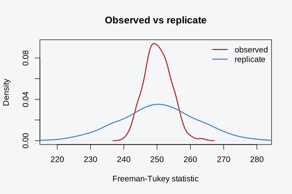

Distributions of the observed and replicate Freeman-Tukey fit statistics, with the observed values sitting above the replicate values

The observed and replicate clouds overlap here, and the Bayesian p-value sits near the middle of its range, which is what a correctly specified model produces. The chi-squared statistic reads the same way.

ppc(fit, fit.stat = "chi-squared")$bayesian.p
#> [1] 0.434

Conditioning the latent state on the detection history is what keeps the p-value calibrated. A site with at least one detection is occupied with probability 1; a site with an all-zero history is occupied with the posterior probability $\psi_i (1 - p_i)^J / [\psi_i (1 - p_i)^J + (1 - \psi_i)]$ . Sampling $z_i$ from the prior $\psi_i$ instead would force a truly occupied but $z_i = 0$ draw to register a large observed discrepancy with no matching replicate term, pulling the p-value toward 0 even when the model is correct. A value far from 0.5 now flags a real misfit: a p-value near 0 means the data are more dispersed than the fit predicts, near 1 means less.

PIT residuals and uniformity

The probability integral transform offers a sharper, per-site view than a single discrepancy statistic collapses into one number. The idea is general. If you evaluate the cumulative distribution function of a correct predictive model at the value it actually observed, the result is uniform on $[0, 1]$ , because that is what running a random variable through its own CDF does. Departures from uniformity are departures of the predictive distribution from the truth, and the shape of the departure names the flaw.

For each site, pit_residuals() treats the ordered detected/all-zero outcome as the response: at least one detection, or none. The predictive CDF at that outcome has two limits – the probability the model places on the all-zero path (the occupied-but-undetected path plus the unoccupied path), and either 1 (a detected site sits above that mass) or 0 (an all-zero site sits below it). A randomized PIT residual is drawn uniformly between those two limits, per site, per posterior draw average – the usual construction for a discrete or mixed response, not an ad hoc jitter. If the model is correct, the resulting values are uniform on $[0, 1]$ .

pit <- pit_residuals(fit)
length(pit); summary(pit)
#> [1] 300
#>     Min.  1st Qu.   Median     Mean  3rd Qu.     Max. 
#> 0.007594 0.252631 0.516891 0.503076 0.749373 0.997724

test_uniformity() runs a Kolmogorov-Smirnov test of the PIT values against the uniform. It returns the standard htest object.

test_uniformity(pit)
#> 
#>  Asymptotic one-sample Kolmogorov-Smirnov test
#> 
#> data:  r
#> D = 0.029863, p-value = 0.9518
#> alternative hypothesis: two-sided

A large p-value, as here, says the PIT values are consistent with uniformity, so the model’s predictive distribution matches the data across the range. The histogram makes the shape concrete.

hist(pit, breaks = 12, col = "grey80", border = "white",
     xlab = "PIT residual", main = "PIT residuals vs uniform")
abline(h = length(pit) / 12, col = "steelblue", lwd = 2, lty = 2)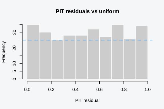

Histogram of PIT residuals lying roughly flat between zero and one, consistent with the uniform reference

The shape of a non-uniform PIT histogram tells you what went wrong, and the mapping is worth committing to memory because it generalises across families. A U-shape, with mass piling up at both ends, means the predictive distribution is too narrow: the data fall in the tails more often than the model expects, the signature of underdispersion. A hump in the middle, the mirror image, means the predictive distribution is too wide and the data cluster nearer the centre than the model allows, the signature of overdispersion. A slope, with mass drifting toward one end, means the predictive mean is biased that way and a covariate or an offset is missing. With a flat histogram, as here, the predictive distribution matches the data across its whole range and there is nothing to chase.

The KS p-value formalises the eye test. It can be conservative when the response is discrete and the jitter leaves ties, which the function handles by suppressing the ties warning while keeping the asymptotic p-value, but the histogram is the part to read first. A test that passes with a histogram that looks wrong is a sign of low power at the current sample size, not a clean bill of health.

Simulation-based calibration

The PIT above asks whether the fitted model predicts the data it saw. A different question sits underneath it: whether the algorithm that produced the posterior is calibrated at all. A fit can predict its own data acceptably while reporting intervals that are systematically too narrow, and no amount of posterior-predictive checking finds that, because both halves of the check come from the same posterior.

Simulation-based calibration answers it by construction. Draw a truth from the distribution the fit updates, simulate a data set at that truth, refit, and record where the truth falls in the new posterior. Under exact inference those ranks are uniform, so the whole rank ECDF is the measurement rather than coverage at one or two nominal levels (Talts et al. 2018). sbc() runs the posterior variant, which draws the truth from the fit’s own posterior at an observed data set and refits on the observed data and the replicate together (Sailynoja et al. 2026). That variant is the one that applies here: the nested-Laplace door puts no prior on the fixed effects, so they cannot be drawn from a prior, while a posterior conditioned on data is proper whatever the prior was.

The fixture is a coupled cover model, the case the method matters most for: occupancy and cover share one areal field, the cover arm sees it through a copy scale alpha, and both are estimated on an outer grid.

N <- 50L; J <- 6L
adj <- matrix(0L, N, N)
for (s in seq_len(N)) {
  if (s > 1L) adj[s, s - 1L] <- 1L
  if (s < N)  adj[s, s + 1L] <- 1L
}
sim <- simulate_occu_cover(N = N, J = J, positive = "lognormal", adj = adj,
                           beta.occ = c(0.2, 0.6), beta.p = c(0.4, -0.5),
                           beta.pos = c(log(0.25), 0.3),
                           sigma = 0.8, alpha = 1.0, sigma.pos = 0.4,
                           seed = 707L)
long <- data.frame(site_id = rep(seq_len(N), each = J),
                   visit = rep(seq_len(J), times = N),
                   y = as.vector(t(sim$y)),
                   det_cov1 = sim$visit_data$det_cov1,
                   pos_cov1 = sim$visit_data$pos_cov1)
od <- tobs_data(long, y = "y", site = "site_id", visit = "visit",
                det.covs = c("det_cov1", "pos_cov1"))
y_pos <- sim$y_pos; y_pos[is.na(y_pos)] <- 0

ctl <- list(engine = "joint", verbose = FALSE,
            sigma.grid    = exp(seq(log(0.15), log(2.0), length.out = 9)),
            phi.grid.pos  = exp(seq(log(0.20), log(0.90), length.out = 7)))
fit <- tobs(~ occ_cov1 + icar(graph = adj),
            data = cbind(data.frame(site_id = seq_len(N)), sim$data),
            family = occu_cover("lognormal"),
            detection = ~ det_cov1,
            positive  = ~ pos_cov1 + share(spatial()),
            y = od$y, y.pos = y_pos, visits = od$det.covs,
            method = "nested_laplace", control = ctl)

Two settings in that control are there for the calibration run rather than for the fit. The dispersion goes on the outer grid so it is estimated: left off it the joint engine fixes it per data set, which would generate the replicate at one value and score it under another. The field-SD grid is pinned because a defaulted axis is re-placed per fit, and a truth drawn from one support scored against a predictive on another measures grid placement instead of calibration.

res <- sbc(fit, n.sim = 100L, n.draws = 1000L, n.ref = 200L,
                controls = "narrow", fit.control = ctl)
res

The run costs one refit per simulation on the pooled data, about 205 seconds for 100 simulations on this fixture. What comes back is a tulpa::sbc object: a rank ECDF per quantity against an exact simultaneous band, the folded read, and the two premises the construction rests on, both reported as verified rather than assumed. controls = "narrow" adds a second arm reporting the same draws with their standard deviation divided by 1.25. It is there because a calibration read that nothing can fail is not evidence.

What is scored is the fixed effects on all three arms, the field standard deviation on each arm, the copy scale alpha, the dispersion, and a rank of a joint statistic over the whole parameter vector. The per-cell field is not scored: it is integrated out by the fit and carries no truth. alpha and the cover-arm field SD are read per draw off the outer grid, whose cells are sampled by their own weight, so what is ranked is the grid-marginalized posterior of each rather than a ratio of component modes.

On this fixture the six arm coefficients and alpha come back uniform, with the smallest p-value over that set at 0.13, while the mis-scaled control reaches 3e-16 on the same quantities and the same fits. alpha alone makes the point: 0.52 as the fit reports it, 3e-16 once its width is distorted.

Two reads leave the band on the correct fit, and they are worth stating plainly. The occurrence-arm field standard deviation puts 81 of 100 ranks in the top decile, and the derived cover-arm SD 87 of 100: the posterior sits systematically low on field scale, or the simulator draws it high. alpha, being a ratio of the two SDs, stays uniform at 0.52, and so do the slopes, which points at a common scale factor rather than at the coupling. The cause is open. Read the field-SD ranks on a pooled fit with that in mind.

Supply model.only = TRUE to get the callback list instead of running the experiment, which is the way to inspect what will be simulated, pooled and refitted before paying for 100 fits.

Dispersion, zero-inflation, and outliers

Three simulation-based tests target specific failure modes. Each draws replicate datasets from the fit with simulate(), computes a feature on the real data and on the replicates, and reports where the data sit. They share a shape: an observed value, an expected value averaged over replicates, a ratio of the two, and a p-value that is the fraction of replicates whose feature meets or exceeds the observed one. Because they simulate from the model rather than redrawing the latent state in isolation, these tests sidestep the calibration issue that affects the omnibus posterior-predictive check, and their p-values are closer to honest tail probabilities. Each one isolates a single named feature, which makes the verdict easy to act on.

test_dispersion() compares the variance of the per-site detection totals against what the model predicts. The ratio is the observed variance over the expected.

test_dispersion(fit)
#> $observed
#> [1] 4.721026
#> 
#> $expected
#> [1] 4.70513
#> 
#> $ratio
#> [1] 1.003378
#> 
#> $p.value
#> [1] 0.468
#> 
#> $alternative
#> [1] "greater"
#> 
#> $sim
#>    sim_1    sim_2    sim_3    sim_4    sim_5    sim_6    sim_7    sim_8 
#> 4.808651 4.855507 4.738194 4.509465 4.769353 4.717949 4.518116 4.641906 
#>    sim_9   sim_10   sim_11   sim_12   sim_13   sim_14   sim_15   sim_16 
#> 4.759465 4.573233 4.368294 4.515619 4.277324 5.314337 4.841695 4.833846 
#>   sim_17   sim_18   sim_19   sim_20   sim_21   sim_22   sim_23   sim_24 
#> 4.819799 4.511427 5.019130 4.762308 4.685574 4.605340 4.989287 4.628082 
#>   sim_25   sim_26   sim_27   sim_28   sim_29   sim_30   sim_31   sim_32 
#> 4.568685 4.635452 4.726544 4.528194 4.750234 4.723567 4.824571 4.874682 
#>   sim_33   sim_34   sim_35   sim_36   sim_37   sim_38   sim_39   sim_40 
#> 4.484103 4.601327 4.656455 4.645920 4.571360 4.462196 4.695608 4.455418 
#>   sim_41   sim_42   sim_43   sim_44   sim_45   sim_46   sim_47   sim_48 
#> 5.011773 4.504738 4.791260 4.890468 4.614314 4.743133 4.968328 4.645440 
#>   sim_49   sim_50   sim_51   sim_52   sim_53   sim_54   sim_55   sim_56 
#> 4.566511 4.601070 5.191572 5.103445 4.814671 4.376042 4.863534 4.738417 
#>   sim_57   sim_58   sim_59   sim_60   sim_61   sim_62   sim_63   sim_64 
#> 4.391026 4.239064 4.892698 5.000792 5.140959 4.793802 5.012531 4.592464 
#>   sim_65   sim_66   sim_67   sim_68   sim_69   sim_70   sim_71   sim_72 
#> 5.263501 5.014983 4.557414 5.043601 5.077492 5.146878 4.851940 4.310758 
#>   sim_73   sim_74   sim_75   sim_76   sim_77   sim_78   sim_79   sim_80 
#> 4.665541 4.677581 4.725574 4.579833 4.759019 4.619889 4.530658 4.592598 
#>   sim_81   sim_82   sim_83   sim_84   sim_85   sim_86   sim_87   sim_88 
#> 4.822029 4.239588 4.863534 4.863534 4.812430 4.007848 4.407258 4.786745 
#>   sim_89   sim_90   sim_91   sim_92   sim_93   sim_94   sim_95   sim_96 
#> 4.315485 4.555452 4.904303 4.181761 4.690123 4.856187 4.646109 4.714604 
#>   sim_97   sim_98   sim_99  sim_100  sim_101  sim_102  sim_103  sim_104 
#> 4.848785 4.926143 4.322007 4.995541 4.378417 4.789788 4.754114 4.596923 
#>  sim_105  sim_106  sim_107  sim_108  sim_109  sim_110  sim_111  sim_112 
#> 4.591695 4.613200 5.270056 5.115541 4.674905 4.609353 4.704247 4.270903 
#>  sim_113  sim_114  sim_115  sim_116  sim_117  sim_118  sim_119  sim_120 
#> 4.864337 4.637681 4.792363 4.466042 5.011137 4.299889 4.842129 4.705139 
#>  sim_121  sim_122  sim_123  sim_124  sim_125  sim_126  sim_127  sim_128 
#> 4.450123 4.938685 4.826522 4.660992 4.993935 4.673032 4.655284 4.642140 
#>  sim_129  sim_130  sim_131  sim_132  sim_133  sim_134  sim_135  sim_136 
#> 4.858417 4.940959 4.939398 5.079420 4.488294 4.694437 4.793969 4.799287 
#>  sim_137  sim_138  sim_139  sim_140  sim_141  sim_142  sim_143  sim_144 
#> 4.700959 4.575017 4.547726 4.771505 4.760970 4.749822 4.227380 4.737748 
#>  sim_145  sim_146  sim_147  sim_148  sim_149  sim_150  sim_151  sim_152 
#> 4.901494 4.155139 4.698718 4.893768 4.460323 4.626745 4.598651 4.451505 
#>  sim_153  sim_154  sim_155  sim_156  sim_157  sim_158  sim_159  sim_160 
#> 4.709431 4.767659 4.702341 5.001962 5.122230 4.717547 4.863980 4.822062 
#>  sim_161  sim_162  sim_163  sim_164  sim_165  sim_166  sim_167  sim_168 
#> 4.454169 4.229420 4.658852 4.591973 4.546477 4.341795 5.227414 4.163880 
#>  sim_169  sim_170  sim_171  sim_172  sim_173  sim_174  sim_175  sim_176 
#> 4.549654 5.169186 4.955407 4.936410 4.949788 4.538361 4.574036 5.452163 
#>  sim_177  sim_178  sim_179  sim_180  sim_181  sim_182  sim_183  sim_184 
#> 4.883779 4.598384 5.281561 4.397715 4.786577 4.536276 4.541628 4.284270 
#>  sim_185  sim_186  sim_187  sim_188  sim_189  sim_190  sim_191  sim_192 
#> 5.109688 5.107815 4.687848 4.300736 4.616009 4.712999 5.050658 4.258763 
#>  sim_193  sim_194  sim_195  sim_196  sim_197  sim_198  sim_199  sim_200 
#> 4.676076 4.712375 4.615151 4.999721 4.734716 4.961828 4.281505 4.970736 
#>  sim_201  sim_202  sim_203  sim_204  sim_205  sim_206  sim_207  sim_208 
#> 5.193133 4.388618 4.582776 4.462609 5.270190 4.958963 5.353969 4.914649 
#>  sim_209  sim_210  sim_211  sim_212  sim_213  sim_214  sim_215  sim_216 
#> 4.618450 4.542430 4.331093 4.919454 4.592408 4.668216 4.749565 4.845039 
#>  sim_217  sim_218  sim_219  sim_220  sim_221  sim_222  sim_223  sim_224 
#> 4.445307 4.928651 4.747146 4.142297 4.903411 4.677547 4.719688 4.224705 
#>  sim_225  sim_226  sim_227  sim_228  sim_229  sim_230  sim_231  sim_232 
#> 4.274203 4.846154 4.290033 4.076020 4.500992 4.490290 4.606143 4.835273 
#>  sim_233  sim_234  sim_235  sim_236  sim_237  sim_238  sim_239  sim_240 
#> 5.188361 4.741405 4.803512 4.764537 4.638517 4.975909 4.990803 4.958428 
#>  sim_241  sim_242  sim_243  sim_244  sim_245  sim_246  sim_247  sim_248 
#> 4.469688 4.317179 4.879320 4.299889 4.603969 4.445975 4.604236 4.413501 
#>  sim_249  sim_250 
#> 4.903668 4.818016

A ratio near 1 and a p-value away from the extremes mean the spread of detections matches the fit. A ratio well above 1 is overdispersion: the detection totals vary more than the model allows, usually because sites differ in occupancy or detection in ways the covariates do not capture, so some sites pile up detections while others stay empty beyond what the fit predicts. The cure is a richer mean structure, a random effect on site, or a spatial field. A ratio well below 1 is the rarer underdispersion, where the data are smoother than the model expects. For counts rather than detections the same diagnostic drives the choice between Poisson and negative binomial abundance: an overdispersion flag on a Poisson N-mixture fit is the standard reason to switch to the negative binomial, covered in the abundance vignette.

test_zero_inflation() counts sites with no detections at all and asks whether the model produces that many all-zero sites.

test_zero_inflation(fit)
#> $observed
#> [1] 126
#> 
#> $expected
#> [1] 126.172
#> 
#> $ratio
#> [1] 0.9986368
#> 
#> $p.value
#> [1] 0.524

The observed count of empty sites matches the expected count, so there is no excess of zeros. This test matters for occupancy because the model already produces zeros two ways, through unoccupied sites and through occupied sites that went undetected, and the question is whether those two sources together account for all the empty sites in the data. An observed value far above the expected, with a p-value near 0, would say they do not: the data have more empty sites than occupancy plus detection can explain. The usual culprits are a third zero-generating process the model omits, such as habitat that is structurally unsuitable, or detection that collapses to near zero at a subset of sites. Either points toward a zero-inflated or hurdle structure, or toward a detection covariate that separates the dead sites from the live ones.

test_outliers() flags sites whose detection total falls outside the central 95% of the replicate distribution, then checks whether the number of such sites is itself surprising.

test_outliers(fit)
#> $observed
#> [1] 2
#> 
#> $expected
#> [1] 1.612
#> 
#> $ratio
#> [1] 1.240695
#> 
#> $p.value
#> [1] 0.456

A handful of outliers is expected by chance; 5% of sites sit outside a 95% interval by construction, so the raw count is not alarming on its own. The p-value does the calibration: it asks whether the count of outliers in the data exceeds what the model produces on its own replicates, which centres the comparison on the model’s own expectation rather than the nominal 5%. A small p-value points to a few sites the model cannot accommodate. Those are worth inspecting individually, because a population-level fit can look fine while a small number of sites with unusual detection histories distort the estimates. Cross-referencing the flagged sites with the largest Pearson residuals from the next section usually identifies the same handful, which is the cue to check them for data-entry errors, unusual survey effort, or a covariate value the model did not see.

Residuals

residuals() returns a list with two elements, because an occupancy model has two processes. $occ is one residual per site, comparing the observed occupancy indicator (any detection) against the fitted occupancy probability. $det is a site-by-visit matrix of detection residuals, with NA where a visit was not made.

r <- residuals(fit, type = "pearson")
length(r$occ)
#> [1] 300
dim(r$det)
#> [1] 300   6

The type argument follows the usual convention. "response" is the raw difference between observed and fitted, on the scale of the data. "pearson" divides that difference by the fitted standard deviation, which standardises sites with different fitted probabilities onto a common scale so that a residual of 2 means the same thing at a rare site and a common one. "deviance" is the signed root of the per-observation deviance contribution, the residual whose sum of squares is the model deviance, and the one whose distribution is closest to normal for binary data. Pearson residuals are the natural default for spotting sites the model handles badly, since the common scale makes large values comparable; deviance residuals are the better choice when you want the residual distribution itself to look normal in a QQ plot.

The two-part return reflects that an occupancy fit predicts two things and can be wrong about either. The occupancy residual asks whether the model got the site’s occupancy probability right given whether it was ever detected. The detection residuals ask, visit by visit, whether the model got the per-visit detection probability right at sites it believes are occupied. A model can fit occupancy well and detection badly, or the reverse, and keeping the two residual streams separate is what lets you tell which.

A residuals-against-fitted plot is the first thing to draw. Structure in the cloud, such as a trend or a fan, signals a misspecified mean or variance. Here the occupancy residuals scatter without pattern.

fv <- fitted(fit)
plot(fv$psi, r$occ, pch = 16, col = rgb(0, 0, 0, 0.35),
     xlab = "fitted occupancy probability", ylab = "Pearson residual (occupancy)")
abline(h = 0, col = "steelblue", lwd = 2)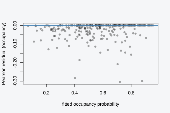

Pearson occupancy residuals plotted against fitted occupancy probability, scattered around zero with no trend

The detection residuals live in the matrix r$det, one row per site and one column per visit, with NA in the cells for visits that were not made. Collapsing them to a per-site mean gives a quick read on which sites contribute the most detection misfit, again with no structure expected under a good model.

det_site <- rowMeans(r$det, na.rm = TRUE)
summary(det_site)
#>     Min.  1st Qu.   Median     Mean  3rd Qu.     Max. 
#> -0.95472 -0.11116 -0.02528 -0.01322  0.09521  0.86808

A per-site mean near zero across the board, as here, says the detection model is not systematically over- or under-predicting at any site. If you suspect a detection covariate is missing, plotting these per-site means against the candidate covariate is the direct check: a trend in that plot is the covariate announcing itself. The same matrix supports a per-visit view, by taking column means instead, which catches a detection process that drifts across the survey season.

Spatial residual diagnostics

When sites carry coordinates, leftover residual structure in space is a sign of a missing spatial field. The reasoning is the same as for a missing covariate. If nearby sites share an unmodelled influence, such as a climate gradient or a dispersal corridor, their residuals will share sign and magnitude, and that shared pattern is detectable even though the influence itself is unobserved. A correctly specified model leaves residuals that are spatially independent, scattered without regard to which sites are neighbours.

The tulpa engine that powers tulpaObs exports two helpers for this, inherited through the fit’s class. moran_i() reduces the spatial pattern to a single autocorrelation statistic and tests it; tulpa_variogram() shows how residual similarity changes with distance, which carries more detail about the range of the structure. Both accept a residual vector directly, so feed them the $occ element from the residual list rather than the whole list.

To show the diagnostic working, simulate occupancy on a grid where the occupancy intercept follows a smooth spatial surface. A model with no spatial term will leave that surface in its residuals.

side   <- 12L
coords <- expand.grid(lon = seq_len(side), lat = seq_len(side))
N      <- nrow(coords)

adj <- matrix(0L, N, N)                     # rook adjacency on the grid
for (i in seq_len(N)) for (j in seq_len(N)) {
  if (i < j &&
      abs(coords$lon[i] - coords$lon[j]) +
      abs(coords$lat[i] - coords$lat[j]) == 1) {
    adj[i, j] <- 1L; adj[j, i] <- 1L
  }
}

field <- 2.2 * sin(coords$lon / 2.2) + 2.2 * cos(coords$lat / 2.2)
xg  <- rnorm(N)
z   <- rbinom(N, 1, plogis(-0.2 + 0.5 * xg + field))
yg  <- matrix(0L, N, 7L)
for (i in seq_len(N)) if (z[i] == 1L) yg[i, ] <- rbinom(7L, 1, 0.6)
datg <- data.frame(x = xg)

Fit two models: a non-spatial Laplace fit that ignores the surface, and a nested-Laplace fit with an intrinsic CAR (icar()) field on the same adjacency graph.

fit_ns <- tobs(~ x, data = datg, family = occu(),
               detection = ~ 1, y = yg, method = "laplace",
               control = list(verbose = FALSE))
fit_sp <- tobs(~ x + icar(graph = adj), data = datg, family = occu(),
               detection = ~ 1, y = yg, method = "nested_laplace",
               control = list(max.iter = 10L, verbose = FALSE))
#> Warning: occu(): the nested_laplace fit stopped after 10 iterations without
#> meeting its convergence criterion, so the estimates are not at the mode. Raise
#> control$max.iter (or loosen control$tol); convergence(fit) has the record.

Moran’s I on the occupancy residuals measures how strongly neighbouring sites share residual sign and size. The function returns an htest with the statistic and a p-value under the randomisation null.

mi_ns <- tulpa::moran_i(residuals(fit_ns)$occ, coords = coords,
                        weights = "knn", k = 8)
mi_sp <- tulpa::moran_i(residuals(fit_sp)$occ, coords = coords,
                        weights = "knn", k = 8)

data.frame(
  model    = c("non-spatial", "icar field"),
  moran_I  = round(c(mi_ns$statistic, mi_sp$statistic), 3),
  p_value  = signif(c(mi_ns$p.value, mi_sp$p.value), 2)
)
#>         model moran_I p_value
#> 1 non-spatial   0.353 2.4e-19
#> 2  icar field   0.057 1.1e-01

Moran’s I runs from roughly $-1$ to $+1$ , with values near its small negative expected value indicating no spatial pattern. The non-spatial fit leaves strong positive autocorrelation in its residuals: neighbouring sites are wrong in the same direction because the shared spatial surface is unmodelled, and the statistic sits far above its expected value with a p-value near zero. Adding the CAR field absorbs most of that structure, and Moran’s I drops sharply toward its null. The field is doing the work the residuals show is needed. The weights argument controls how neighbours are defined: "knn" with a chosen k uses the k nearest sites, while "inverse" weights every pair by inverse distance. The k-nearest choice is the steadier one on a regular grid, since it does not let a few close pairs dominate the statistic.

The variogram tells the same story as a curve, with the advantage that it shows the range over which the structure operates rather than collapsing it to one number. It bins pairs of sites by distance and plots half the mean squared residual difference in each bin, the semivariance. Under spatial structure, nearby sites have similar residuals and the semivariance is small at short distances, rising as distance grows until pairs are far enough apart to be effectively independent, where the curve levels off. The distance at which it levels is the range of the residual structure, which tells you roughly how far a spatial field would need to reach. A flat curve across all distances means no structure is left.

vg <- tulpa::tulpa_variogram(residuals(fit_ns)$occ, coords = coords)
plot(vg)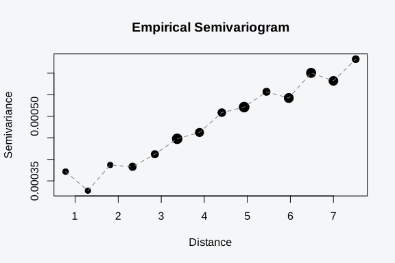

Empirical semivariogram of non-spatial occupancy residuals rising with distance before levelling, indicating residual spatial structure

The rise in the non-spatial residual variogram confirms the Moran’s I verdict. If you compute the same curve on the spatial fit’s residuals, it flattens, which is the visual form of the autocorrelation shrinking. Both helpers also accept a fitted model directly and call residuals() for you, but the tobs residual list means passing the $occ vector is the safe route.

Prior specification and its effect on the fit

The Laplace fit carries a weakly-informative prior by default, and it is part of the diagnostic story because it changes the numbers a check reads. The unpenalised occupancy MAP sits on the psi-p identifiability ridge when visits are few: with a handful of revisits per site, “unoccupied” and “occupied but never detected” look almost the same from the data alone, and the likelihood flattens along the direction that trades one for the other. NUTS escapes the ridge through its prior; an unpenalised Laplace fit does not, and its detection coefficients can drift far with large standard errors. occu_priors() builds the penalty that breaks the ridge, a Normal prior on each coefficient group.

occu_priors()
#> occu_priors (weakly-informative for method='laplace'):
#>   p_(Intercept) ~ Normal(0, 1.5)
#>   p slopes       ~ Normal(0, 2.5)
#>   psi_(Intercept) ~ Normal(0, 2)
#>   psi slopes     ~ Normal(0, 5)

The four buckets cover the detection intercept (sd = 1.5), detection slopes (sd = 2.5), occupancy intercept (sd = 2), and occupancy slopes (sd = 5). The detection side is tighter because that is where the ridge bites; the occupancy side is looser because occupancy is identified more directly by which sites ever detect. To see the prior at work, build a low-information dataset with only three visits per site, where the ridge is sharp, and fit it both with the default prior and with priors = FALSE to recover the unpenalised MAP.

sim3 <- simulate_occu(N = 120, J = 3, n.occ.covs = 1, n.det.covs = 1,
                      beta.occ = c(0.3, 1.0), beta.det = c(0.0, 0.8), seed = 7)
fit_pen   <- tobs(~ occ_cov1, data = sim3$data, family = occu(),
                  detection = ~ det_cov1, y = sim3$y, method = "laplace",
                  control = list(verbose = FALSE))
fit_unpen <- tobs(~ occ_cov1, data = sim3$data, family = occu(),
                  detection = ~ det_cov1, y = sim3$y, method = "laplace",
                  priors = FALSE, control = list(verbose = FALSE))

Line up the detection-intercept estimate and its standard error from the two fits against the truth of 0.0. The penalised fit holds the estimate near zero with a controlled standard error; the unpenalised fit, free to slide along the ridge, returns a larger magnitude and a wider interval.

data.frame(
  fit  = c("penalised", "unpenalised"),
  p_int = round(c(fit_pen$means["p_(Intercept)"],
                  fit_unpen$means["p_(Intercept)"]), 3),
  se    = round(c(fit_pen$sds[["p_(Intercept)"]],
                  fit_unpen$sds[["p_(Intercept)"]]), 3)
)
#>           fit p_int    se
#> 1   penalised 0.192 0.184
#> 2 unpenalised 0.194 0.186

The prior is doing identification work, not imposing a result. At moderate information, more visits or a stronger detection signal, the two fits converge because the likelihood pins the coefficient and the prior barely registers; the gap above is a small-J phenomenon. Setting any bucket’s sd to Inf removes the penalty on that group while keeping the others, so you can penalise only the detection side that needs it. The diagnostic reading is that a detection coefficient with an implausibly large magnitude and a standard error to match, on a fit with few visits, is the ridge showing through, and the default prior is the first thing to confirm is in place before chasing the estimate as a substantive finding.

A diagnostic workflow

The checks fall into an order that catches the cheap problems first and spends simulation effort only once the cheap checks pass. The first two steps cost nothing beyond the fit you already have. The middle steps simulate from the model, which takes a few seconds. The spatial step needs coordinates and a second fit. Running them in this order means you rarely pay for the expensive checks on a model that a cheap check would have rejected.

Run check_model() for a first pass. The one-call panel prints the WAIC, the PPC p-value, the zero-inflation count, and, with coords, the Moran’s I, each with a warning band. A clean panel means the detailed steps are confirmation; a warning means open the matching section.
Read the coefficients against their intervals. A coefficient whose credible interval spans zero is not earning its place, whatever its point estimate. Start with summary() and confint(). On a fit with few visits, an outsized detection coefficient is the identifiability ridge, not a finding; confirm the default occu_priors() is in place.
Compare against nested alternatives with waic(). Drop the covariate, add a plausible one, and read the delta. A change of a few units or less is a tie; prefer the simpler model. WAIC ranks, it does not validate.
Run a posterior-predictive check with ppc(). The Bayesian p-value sits near 0.5 for a fit that reproduces the data. A value near 0 means the data are more dispersed than the fit predicts, near 1 means less. The check conditions the latent state on the detection history, so the value is calibrated rather than purely relative.
Inspect the PIT histogram and test_uniformity(). A flat histogram is the target. A U-shape means underdispersion, a central hump overdispersion, a slope a biased mean.
Target specific failures. test_dispersion() for spread, test_zero_inflation() for excess empty sites, test_outliers() for individual sites the model cannot fit.
Plot residuals against fitted values. Structure in the cloud points to a misspecified mean or variance. Use Pearson residuals for a common scale.
If sites have coordinates, test for residual spatial structure with moran_i() and tulpa_variogram() on residuals(fit)$occ. Significant autocorrelation is the cue to add a spatial field and refit, then confirm the autocorrelation shrinks.

The point throughout is that a clean coefficient table is necessary and not sufficient. The fit earns trust when it survives the checks, and each check that fails names the next term to add: a dispersion flag asks for a random effect, a zero-inflation flag for a hurdle or a detection covariate, a spatial-autocorrelation flag for a field. Diagnostics are not a final exam the model either passes or fails. They are the loop that turns a first fit into a defensible one, and the most useful outcome of a failed check is the specific term it tells you to add before the next pass.

Where to go next

The accessors behind these checks, coef(), summary(), confint(), fitted(): vignette("occupancy").
Model comparison by marginal likelihood at the engine level, and what WAIC and LOO need: the tulpa model-comparison vignette.
Adding spatial fields once the residual diagnostics call for them: vignette("occupancy") and the spatial model vignettes.
Dispersion in counts, where the negative binomial answers an overdispersion flag: vignette("abundance"). ```