Dynamic (multi-season) occupancy

Installation

install.packages("pak")
pak::pak("gcol33/tulpaObs")            # latest from GitHub
pak::pak("gcol33/tulpaObs@v0.1.1")     # a specific tagged release

Tagged releases are listed at https://github.com/gcol33/tulpaObs/releases.

pak resolves the dependency tree, pulling tulpa and tulpaMesh from the r-universe repository DESCRIPTION declares in Additional_repositories, at or above the Imports floor. A C++17 toolchain is needed (Rtools on Windows, Xcode CLI tools on macOS, r-base-dev on Linux); both tulpa and tulpaObs compile their backends on first install.

library(tulpaObs)
library(ggplot2)

transparent <- theme(
  panel.background = element_rect(fill = "transparent"),
  plot.background  = element_rect(fill = "transparent")
)

When occupancy changes over time

A single-season occupancy model treats a site as either occupied or empty and asks only whether you detected the species. That picture holds for a snapshot. Run the same survey for several years and the picture moves: a pond that was empty fills with frogs, a meadow loses its butterflies, a forest patch is colonised and then goes quiet again. The state itself is no longer fixed. It is a sequence, and the interesting questions are about the changes between the entries in that sequence.

Two rates govern those changes. Colonisation is the chance that an empty site becomes occupied by the next season. Local extinction is the chance that an occupied site becomes empty. A site’s trajectory is a chain of occupied and empty states linked by these two rates, and the species is detected only when the site is occupied and you happen to catch it on a visit. The dynamic occupancy model of MacKenzie and colleagues separates all three pieces: where the species starts, how it moves between states, and how often you see it when it is there.

The reason to separate them is that the raw data hide all three behind the same zeros. A site that records no detections in a season might be empty, or occupied but missed. A site occupied this year but not last might have been colonised, or might have been occupied all along and undetected the first year. Detection error and state change both turn a present species into a string of zeros, and only a model that names the two processes can tell which zeros are which. The dynamic model layers a detection process over a Markov chain on the state and estimates the rates of each from the pattern of zeros and ones across visits and seasons.

dyn_occu() fits that model in tulpaObs. You hand it a detection history with a season dimension, a formula for first-season occupancy, a formula for colonisation, a formula for extinction, and a detection formula. This vignette simulates a known trajectory, fits it, checks that the rates come back, derives turnover and the long-run occupancy the rates imply, and works through when the rates are identifiable and when they are not.

The model

Let $z_{i,t}$ be the latent occupancy state of site $i$ in season $t$, equal to $1$ if the species is present and $0$ if not. The first season is drawn from an initial occupancy probability,

$$z_{i,1} \;\sim\; \mathrm{Bernoulli}(\psi_1),$$

and every later season follows from the one before it through colonisation $\gamma$ and extinction $\epsilon$,

$$z_{i,t} \mid z_{i,t-1} \;\sim\; \begin{cases} \mathrm{Bernoulli}(1 - \epsilon) & z_{i,t-1} = 1 \\[2pt] \mathrm{Bernoulli}(\gamma) & z_{i,t-1} = 0. \end{cases}$$

An occupied site stays occupied with probability $1 - \epsilon$ and goes empty with probability $\epsilon$. An empty site is colonised with probability $\gamma$ and stays empty with probability $1 - \gamma$. Those four numbers are a $2 \times 2$ transition matrix on the state, with rows indexed by last season’s state and columns by this season’s,

$$T \;=\; \begin{pmatrix} 1 - \gamma & \gamma \\ \epsilon & 1 - \epsilon \end{pmatrix},$$

where the first row starts empty and the second row starts occupied. The state sequence $z_{i,1}, z_{i,2}, \dots$ is a two-state Markov chain: the next state depends on the present one and nothing earlier. This is the hidden part of a hidden Markov model, hidden because you never see $z$ directly.

Reading the matrix row by row recovers the two rates. The empty row, $(1 - \gamma,\ \gamma)$, says an empty site stays empty unless it is colonised. The occupied row, $(\epsilon,\ 1 - \epsilon)$, says an occupied site stays occupied unless it goes extinct. The columns of any one row sum to one because the site must land in one of the two states. Multiplying a row vector of occupancy probabilities by $T$ advances it one season, which is the recipe the trajectory section uses to draw the modelled curve forward.

Detection is the observation layer on top of the chain. On visit $j$ of season $t$ you record $y_{i,j,t} = 1$ if you saw the species and $0$ if not, and a sighting is possible only when the site is occupied,

$$y_{i,j,t} \mid z_{i,t} \;\sim\; \mathrm{Bernoulli}(z_{i,t}\, p),$$

so an empty site produces only zeros and an occupied site produces a $1$ with probability $p$ on each visit. A season of all-zero visits is therefore ambiguous: the site was empty, or it was occupied and you missed the species every time. The model resolves that ambiguity in two directions at once. Within a season the repeat visits separate a true absence from a run of misses, since an occupied site with detection $p$ produces at least one sighting in $J$ visits with probability $1 - (1 - p)^J$. Across seasons the transition rates tie a site’s silent year to its neighbours in time, so a site detected before and after a blank season is judged more likely to have been occupied throughout than one blank at the end of its record.

tulpaObs sums the latent chain out with the forward algorithm, the standard recursion for a hidden Markov model. It carries forward the probability of the detection history up to season $t$ jointly with each possible current state, multiplies by the transition matrix to step to season $t + 1$, and folds in that season’s detections. Summing over the two states at the end gives the likelihood of the whole history with $z$ integrated out, so the latent states never appear as parameters and the likelihood is a function of $\psi_1, \gamma, \epsilon, p$ alone. This is why the fit returns four rates rather than a state for every site and season.

Each of those four can carry its own linear predictor. By default they are intercept-only, fitted on the logit scale and reported back as probabilities, but gamma and epsilon accept covariate formulas the same way occupancy and detection do, which is the subject of a later section.

Simulating a trajectory

simulate_dyn_occu() builds a dataset with a known initial occupancy, known colonisation and extinction rates, and a known detection probability, so the fit has a truth to recover. The arguments gamma and epsilon are the colonisation and extinction probabilities directly; beta.occ and beta.det are logit-scale intercepts, so beta.occ = c(0) means $\psi_1 = 0.5$ and beta.det = c(0) means $p = 0.5$.

sim <- simulate_dyn_occu(
  N = 200, J = 4, n.seasons = 6,
  beta.occ = c(0),    # psi1 = plogis(0) = 0.5
  beta.det = c(0),    # p    = plogis(0) = 0.5
  gamma    = 0.3,     # colonisation: empty -> occupied
  epsilon  = 0.2,     # extinction:   occupied -> empty
  seed     = 2026
)
str(sim, max.level = 2)
#> List of 3
#>  $ y    : int [1:200, 1:4, 1:6] 0 0 1 0 0 0 0 0 0 0 ...
#>  $ data :'data.frame':   200 obs. of  1 variable:
#>   ..$ x: num [1:200] 0.5206 -1.0797 0.1392 -0.0847 -0.6666 ...
#>  $ truth:List of 10
#>   ..$ psi1           : num 0.5
#>   ..$ p              : num 0.5
#>   ..$ gamma          : num 0.3
#>   ..$ epsilon        : num 0.2
#>   ..$ beta_gamma     : NULL
#>   ..$ beta_epsilon   : NULL
#>   ..$ beta_det_season: NULL
#>   ..$ z              : num [1:200, 1:6] 0 0 1 0 0 0 0 0 0 1 ...
#>   ..$ beta_occ       : num 0
#>   ..$ beta_det       : num 0

The response sim$y is a three-dimensional array indexed by site, visit, and season. The third dimension is what makes the model dynamic; a two-dimensional matrix would be a single-season detection history and dyn_occu() rejects it.

dim(sim$y)             # 200 sites x 4 visits x 6 seasons
#> [1] 200   4   6
sim$y[1, , ]           # one site: rows are visits, columns are seasons
#>      [,1] [,2] [,3] [,4] [,5] [,6]
#> [1,]    0    0    0    0    1    0
#> [2,]    0    0    0    0    0    0
#> [3,]    0    0    0    0    1    1
#> [4,]    0    1    0    0    1    1

A missing visit is encoded as NA and dropped from that season’s detection count, so seasons can carry different numbers of visits and a site can be unvisited in some seasons without breaking the chain. The state still transitions across a season with no data; the model simply has nothing to update detection with for that cell, and the transition rates carry the occupancy forward. This is what lets the model handle the ragged survey effort real monitoring programmes produce, where not every site is visited every year.

The truth list carries the latent state matrix sim$truth$z, one row per site and one column per season, which the fit never sees. Averaging it down the columns shows the realised occupancy in each season. With colonisation above extinction, occupancy climbs from its starting value toward a higher level and then settles.

occ_by_season <- colMeans(sim$truth$z)
round(occ_by_season, 3)
#> [1] 0.455 0.580 0.580 0.555 0.560 0.580
traj <- data.frame(season = seq_along(occ_by_season), occ = occ_by_season)
ggplot(traj, aes(season, occ)) +
  geom_hline(yintercept = 0.3 / (0.3 + 0.2), colour = "steelblue",
             linewidth = 1, linetype = 2) +
  geom_line() + geom_point(size = 2) +
  ylim(0, 1) + labs(x = "season", y = "occupied fraction") + transparent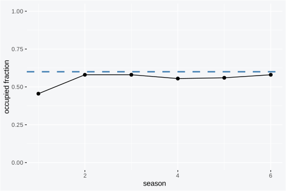

The dashed line marks $\gamma / (\gamma + \epsilon) = 0.6$, the occupancy the two rates pull the system toward in the long run. The realised fraction wobbles around it because two hundred sites is a finite sample of a stochastic chain, not because the rates are drifting. A site’s own path is a string of occupied and empty seasons; the population fraction is the average over those strings.

The ecological reading of the two rates is worth stating before fitting. A high $\gamma$ describes a species that spreads readily into empty habitat: good dispersal, abundant propagules, vacant patches that are easy to reach. A high $\epsilon$ describes a species that blinks out of occupied patches easily: small local populations, harsh between-season conditions, habitat that degrades. The balance between them sets whether a metapopulation grows, shrinks, or holds steady, and the ratio sets the level it holds at.

The two rates also separate processes that a single occupancy number blurs together. Suppose occupancy holds at sixty percent across a decade. That same stable level can come from a placid system where the same sites stay occupied year after year, or from a churning one where many sites wink out each season and just as many are colonised. The static occupancy is identical; the dynamics are opposite, and they imply different conservation responses. Estimating $\gamma$ and $\epsilon$ rather than occupancy alone is what tells the two apart, and it is the reason a multi-season survey is worth the extra effort over repeating a single-season one.

Fitting

The call mirrors the single-season one with two extra formulas. The first argument is the first-season occupancy formula $\psi_1$, detection is the per-visit detection formula $p$, and colonization and extinction are the colonisation $\gamma$ and extinction $\epsilon$ formulas. All four are intercept-only here. The response is the three-dimensional array, and method = "laplace" is the default.

fit <- tobs(
  ~ 1,                                 # psi1: first-season occupancy
  data        = sim$data,
  family      = dyn_occu(),
  detection   = ~ 1,                   # p: per-visit detection
  y           = sim$y,
  colonization = ~ 1,                   # gamma: colonisation
  extinction = ~ 1,                   # epsilon: extinction
  method      = "laplace",
  control     = list(verbose = FALSE)  # the EM prints its iterations otherwise
)
fit
#> <tobs_fit: dynamic occupancy (HMM)>
#>   family         : dyn_occu (status: working)
#>   default method : laplace
#> 
#>   Sites: 200, Seasons: 6, Max visits: 4
#>   Samples: 1000
#> 
#> Mean initial occupancy (intercept): 0.471
#> Mean detection (intercept): 0.501
#> Mean colonization (intercept): 0.299
#> Mean extinction (intercept): 0.210

The response array must be three-dimensional. Passing a flat matrix, the shape a single-season model expects, raises an error that names the requirement rather than fitting the wrong model silently.

tobs(~ 1, data = sim$data, family = dyn_occu(), detection = ~ 1,
     y = sim$y[, , 1],                 # a single season: 2D matrix
     colonization = ~ 1, extinction = ~ 1,
     control = list(verbose = FALSE))
#> Error in `.tobs_build_dynamic()`:
#> ! y must be a 3D array [n_sites x max_visits x n_seasons] or a list of matrices

The fitted object holds the four rates back-transformed to the probability scale in $intercepts. This is the quickest read of the result: where occupancy starts, how fast empty sites fill, how fast occupied sites empty, and how often a present species is seen.

fit$intercepts
#> $psi1
#> psi1_(Intercept) 
#>        0.4709663 
#> 
#> $p
#> p_(Intercept) 
#>     0.5012209 
#> 
#> $gamma
#> gamma_(Intercept) 
#>         0.2985127 
#> 
#> $epsilon
#> epsilon_(Intercept) 
#>           0.2100606

The values land near the simulated truth of $\psi_1 = 0.5$, $\gamma = 0.3$, $\epsilon = 0.2$, and $p = 0.5$. coef() returns the same four processes on the logit scale, the scale the linear predictors live on, each name prefixed by its process.

coef(fit)
#>    psi1_(Intercept)       p_(Intercept)   gamma_(Intercept) epsilon_(Intercept) 
#>        -0.116265609         0.004883729        -0.854390549        -1.324560099

summary() adds the posterior standard deviation and credible bounds for every coefficient, with the process prefix on each row: psi1_ for first-season occupancy, p_ for detection, gamma_ for colonisation, and epsilon_ for extinction.

summary(fit)
#>                         estimate  std.error       2.5 %     97.5 %
#> psi1_(Intercept)    -0.116265609 0.15045050 -0.41114317  0.1786120
#> p_(Intercept)        0.004883729 0.04499025 -0.08329554  0.0930630
#> gamma_(Intercept)   -0.854390549 0.11038364 -1.07073851 -0.6380426
#> epsilon_(Intercept) -1.324560099 0.12327898 -1.56618246 -1.0829377

Recovering the rates

A model passing its plumbing checks is not the same as a model returning the right numbers. The honest test is to compare the back-transformed rates against the truth they were simulated from. Putting them side by side shows each estimate within a few hundredths of its target.

truth <- c(psi1 = sim$truth$psi1, gamma = sim$truth$gamma,
           epsilon = sim$truth$epsilon, p = sim$truth$p)
est   <- c(psi1 = fit$intercepts$psi1, gamma = fit$intercepts$gamma,
           epsilon = fit$intercepts$epsilon, p = fit$intercepts$p)

data.frame(
  parameter = names(truth),
  truth     = round(truth, 3),
  estimate  = round(est, 3),
  abs_error = round(abs(est - truth), 3),
  row.names = NULL
)
#>   parameter truth estimate abs_error
#> 1      psi1   0.5    0.471     0.029
#> 2     gamma   0.3    0.299     0.001
#> 3   epsilon   0.2    0.210     0.010
#> 4         p   0.5    0.501     0.001

All four absolute errors sit below the tolerance the package test asserts for this regime. Recovery this clean rests on the design: two hundred sites give the chain room to express both transitions, six seasons give five transition steps to estimate the rates from, and four visits per season with detection near one half keep $p$ separated from the occupancy states. Thin any of those and the rates start trading off against one another, the subject of the practical guidance below.

The recovery check is worth running as a habit, not just once. Simulating from the rates you intend to report, fitting, and confirming the estimates return is the cheapest way to learn whether a given survey design can estimate the quantities you care about before you collect the data. If the rates come back biased or with intervals too wide to be useful in the simulation, no analysis of the real data will rescue them; the information was never in the design. The gap between an estimate and its truth here is a few hundredths because the design is generous. A design with three seasons and two visits would show a wider gap and warn you off before fieldwork.

Checking the fit

Recovering the simulated rates shows the fitter can find the truth when the truth matches the model. It says nothing about whether the model matches the data in front of you, which on a real survey is the only question that has no answer key. Three checks come at that question from different angles: an information criterion that scores predictive accuracy, the smoothed state posterior compared against what the model implies, and the per-site-season residuals.

waic() computes the widely applicable information criterion from the pointwise marginal log-likelihood. For a dynamic fit that pointwise term is the forward-algorithm likelihood of each site’s whole detection history with the latent chain summed out, so the score measures how well the model predicts the detection records you saw rather than the unobservable state sequence. A single WAIC means little on its own; it earns its keep in the comparison section below, against a simpler model on the same data.

w <- waic(fit)
c(waic = round(w$estimates["waic", "Estimate"], 1), elpd = round(w$estimates["elpd_waic", "Estimate"], 1), p_waic = round(w$estimates["p_waic", "Estimate"], 2))
#>    waic    elpd  p_waic 
#>  4828.5 -2414.2     4.1

The elpd is the expected log pointwise predictive density, higher meaning a better predictor of new histories of the same shape; p_waic is the effective number of parameters read from how much the pointwise log-likelihood varies across the posterior, which sits near the four rates plus a little slack; and waic is -2 * elpd on the deviance scale, so lower is better and it reads like an AIC with an estimated rather than counted penalty.

The smoothed state posterior gives a second, more direct check. fitted() returns the forward-backward smoothed $P(z_{i,t} = 1 \mid y_{i,1:T})$ as a site-by-season matrix, the model’s belief about occupancy at every cell after seeing the whole record. Any season with a detection smooths to one because a sighting proves presence; a silent season inherits a probability between zero and one from the rates and its neighbours in time. Comparing the column means of that matrix against the realised occupancy from the hidden truth shows the smoothed states tracking the simulation season by season.

fv  <- fitted(fit)
chk <- data.frame(
  truth    = colMeans(sim$truth$z),
  smoothed = colMeans(fv$z)
)
ggplot(chk, aes(truth, smoothed)) +
  geom_abline(slope = 1, intercept = 0, colour = "steelblue", linewidth = 1) +
  geom_point(size = 3) +
  labs(x = "realised occupied fraction", y = "smoothed P(z = 1)") + transparent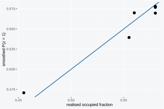

The points hug the identity line, so the per-season smoothed occupancy lands where the truth put it. On a real dataset there is no truth column, but the same matrix is still the honest layer to map: it carries the per-cell uncertainty the rates and the detection history imply rather than collapsing every silent season to a flat zero.

The residuals localise any misfit. residuals() returns an occupancy component shaped like the smoothed z matrix, one residual per site and season comparing the ever-detected indicator at that cell against the smoothed state, with NA where a cell had no visits. Deviance residuals are the default and the natural scale for binary outcomes.

res <- residuals(fit, type = "deviance")
rd  <- data.frame(z = as.vector(fv$z), r = as.vector(res$occ))
rd  <- rd[is.finite(rd$r), ]
ggplot(rd, aes(z, r)) +
  geom_hline(yintercept = 0, colour = "grey50") +
  geom_point(alpha = 0.3) +
  labs(x = "smoothed P(z = 1)", y = "occupancy deviance residual") + transparent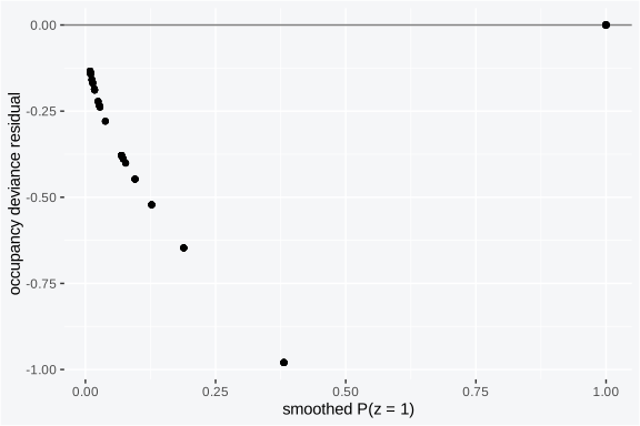

A residual cloud with no trend against the smoothed state, as here, says the state structure is adequate across the range of fitted probabilities. A funnel opening toward one end, or a band that drifts off zero, would point to a rate that varies with something the constant-rate model leaves out, the cue to add a covariate to colonisation or extinction. The posterior-predictive machinery (ppc(), the dispersion and zero-inflation tests) is wired for the single-season detection-history shape and does not run on the three-dimensional dynamic array, so the WAIC, the smoothed-state comparison, and the residuals are the dynamic model’s fit checks.

Turnover and equilibrium occupancy

The two transition rates imply quantities that are often more interesting than the rates themselves. The first is the equilibrium occupancy, the level the metapopulation settles at once the initial condition washes out. Setting the season-to-season change to zero in the transition matrix gives

$$\psi_{\mathrm{eq}} \;=\; \frac{\gamma}{\gamma + \epsilon},$$

the fraction of sites occupied when colonisation and extinction balance. Reading it off the fitted rates gives a number close to the dashed line in the trajectory plot.

g <- fit$intercepts$gamma
e <- fit$intercepts$epsilon
psi_eq <- g / (g + e)
c(psi_eq = round(psi_eq, 3), truth = round(0.3 / (0.3 + 0.2), 3))
#> psi_eq.gamma_(Intercept)                    truth 
#>                    0.587                    0.600

The second is turnover, the share of the occupied set that is made up of newly colonised sites rather than holdovers from the previous season. At equilibrium it works out to

$$\tau \;=\; \frac{\gamma\,(1 - \psi_{\mathrm{eq}})}{\psi_{\mathrm{eq}}} \;=\; \frac{\gamma\,\epsilon}{\gamma + \epsilon}\Big/\psi_{\mathrm{eq}},$$

the colonisation flow into empty sites divided by the equilibrium occupied fraction. A high turnover marks a restless metapopulation whose occupied set is constantly being rebuilt; a low turnover marks a stable one where the same sites stay occupied year after year.

turnover <- (g * (1 - psi_eq)) / psi_eq
round(turnover, 3)
#> gamma_(Intercept) 
#>              0.21

A turnover of this size means a meaningful share of the occupied sites in any season are recent arrivals rather than long-term residents. Two metapopulations can sit at the same equilibrium occupancy with very different turnover: a low-$\gamma$, low-$\epsilon$ system holds the same sites for years, while a high-$\gamma$, high-$\epsilon$ system reshuffles its occupied set constantly even as the headline occupancy stays put. Turnover is the quantity that distinguishes them, and it is invisible to a single-season survey. Reporting it alongside the equilibrium gives a reader both the level the system holds at and the rate at which the membership of that level churns.

The expected occupancy trajectory follows from iterating the transition once per season starting from $\psi_1$. Each season’s occupancy is last season’s pushed through the two rates,

$$\psi_{t} \;=\; \psi_{t-1}(1 - \epsilon) + (1 - \psi_{t-1})\,\gamma,$$

so the modelled curve can be drawn forward from the fitted $\psi_1$, $\gamma$, and $\epsilon$ and laid over the realised fractions from the simulation.

A point trajectory hides the uncertainty in the rates that drive it. The posterior draws make that uncertainty explicit: iterate the recursion once per draw, using that draw’s $\psi_1$, $\gamma$, and $\epsilon$, and the spread of the resulting curves at each season is the credible band on the modelled occupancy. This is the marginalise-the-derived-quantity move applied to a trajectory, propagating the rate posterior through the nonlinear recursion rather than plugging in point estimates.

n_seasons <- dim(sim$y)[3]
dr <- fit$draws
psi_draws <- function(b) {
  pt <- numeric(n_seasons); pt[1] <- plogis(b["psi1_(Intercept)"])
  gg <- plogis(b["gamma_(Intercept)"]); ee <- plogis(b["epsilon_(Intercept)"])
  for (t in 2:n_seasons) pt[t] <- pt[t - 1] * (1 - ee) + (1 - pt[t - 1]) * gg
  pt
}
curves <- t(apply(dr, 1, psi_draws))
band <- data.frame(
  season = seq_len(n_seasons), mean = colMeans(curves),
  lo = apply(curves, 2, quantile, 0.025), hi = apply(curves, 2, quantile, 0.975),
  truth = colMeans(sim$truth$z)
)

ggplot(band, aes(season, mean)) +
  geom_ribbon(aes(ymin = lo, ymax = hi), alpha = 0.2) +
  geom_hline(yintercept = psi_eq, colour = "steelblue", linewidth = 1, linetype = 2) +
  geom_line(colour = "darkorange", linewidth = 1) +
  geom_point(aes(y = truth), size = 2) +
  ylim(0, 1) + labs(x = "season", y = "occupied fraction") + transparent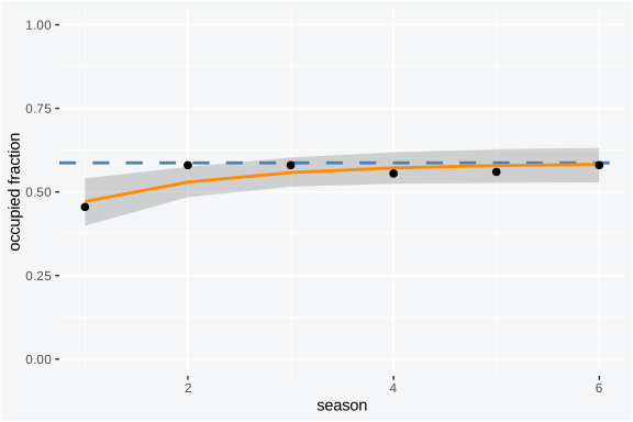

The modelled curve rises from the fitted starting occupancy toward the equilibrium line and the realised fractions sit inside the band across the six seasons. The band is widest in the middle seasons, where the rate uncertainty has had a step or two to compound but the curve has not yet been pinned to the equilibrium it converges on. The gap between the orange curve and the points is sampling noise in two hundred finite chains, not a failure of fit; the curve is the expectation those chains scatter around, and the shaded region is how firmly the rates pin that expectation.

The same draws give a credible interval on the derived equilibrium, computed by evaluating $\gamma / (\gamma + \epsilon)$ on every draw and taking the quantiles, rather than reading a single ratio off the point estimates.

gd <- plogis(dr[, "gamma_(Intercept)"]); ed <- plogis(dr[, "epsilon_(Intercept)"])
eq_draws <- gd / (gd + ed)
round(quantile(eq_draws, c(0.025, 0.5, 0.975)), 3)
#>  2.5%   50% 97.5% 
#> 0.532 0.586 0.637

The interval straddles the true equilibrium of 0.6 and its width reports how much the rate uncertainty leaves open about the level the metapopulation settles at. A point ratio of the two modal rates would land in the middle of this interval and hide its width, which is why the derived equilibrium is worth reporting with the band the draws carry rather than as a bare number.

The speed of approach is itself informative. The distance to equilibrium shrinks by a factor of $1 - \gamma - \epsilon$ each season, so when the two rates are small the system creeps toward its level over many seasons, and when they are large it snaps there in one or two. Here $\gamma + \epsilon = 0.5$, so the curve covers half its remaining distance to the line each season and arrives quickly. A survey that opens far from equilibrium and runs only a few seasons will see occupancy still in transit, which is exactly the case where reporting a single average occupancy across seasons would mislead and the rates carry the real story.

Covariates on colonisation and extinction

Colonisation and extinction need not be constant across sites. A patch near an occupied source colonises faster; a small or exposed patch goes extinct more often. colonization and extinction take covariate formulas exactly as the occupancy and detection formulas do, so a site-level predictor enters the rate on its logit scale. Add a covariate to the data and put it on the colonisation formula.

dat_cov <- sim$data
dat_cov$connectivity <- rnorm(nrow(dat_cov))   # a site-level predictor

fit_cov <- tobs(
  ~ 1,
  data        = dat_cov,
  family      = dyn_occu(),
  detection   = ~ 1,
  y           = sim$y,
  colonization = ~ connectivity,                # colonisation varies by site
  extinction = ~ 1,
  method      = "laplace",
  control     = list(verbose = FALSE)
)
coef(fit_cov, arm = "gamma")
#>  (Intercept) connectivity 
#>  -0.85891068  -0.05577635

The colonisation process now has an intercept and a connectivity slope on the logit scale. The slope is near zero here because connectivity was drawn independently of the simulated trajectory; in a real dataset it would carry the effect of the predictor on the colonisation rate. Extinction takes a formula the same way through extinction, and the two can carry different covariates. To read a fitted rate at a given covariate value, push the logit-scale linear predictor through plogis(); the intercept-only $intercepts shortcut applies only when the formula is ~ 1.

Covariates on the transitions answer questions the constant-rate model cannot. A connectivity covariate on colonisation tests whether patches near occupied sources fill faster, the signature of dispersal limitation. A patch-area covariate with a negative slope on extinction tests whether larger patches hold their populations longer, the signature of demographic rescue. Because each rate carries its own formula, you can let colonisation depend on the landscape between patches and extinction depend on conditions within them, which matches how the two processes actually differ: one is about reaching empty habitat, the other about persisting in occupied habitat. The first-season occupancy formula and the detection formula accept covariates in the same way, so every layer of the model can be made a function of site or visit attributes without changing the call shape.

Prediction

Prediction for a dynamic model has two parts: where occupancy starts at a site you describe with covariates, and where it goes once the transition rates push it forward. The first uses the same machinery the single-season model does. predict(fit, X.0 = ) evaluates the first-season occupancy $\psi_1$ at an explicit design matrix with one column per $\psi_1$ coefficient, the intercept first, and propagates the fixed-effect posterior through to a mean, a standard deviation, and credible bounds at each new row. To make the design carry a covariate, fit $\psi_1$ on a site predictor.

dat_pred <- sim$data
dat_pred$elev <- rnorm(nrow(dat_pred))     # a site-level predictor on psi1

fit_pred <- tobs(
  ~ elev,                                  # first-season occupancy varies by site
  data        = dat_pred,
  family      = dyn_occu(),
  detection   = ~ 1,
  y           = sim$y,
  colonization = ~ 1,
  extinction = ~ 1,
  method      = "laplace",
  control     = list(verbose = FALSE)
)

The columns of X.0 line up with the $\psi_1$ coefficients in order, the intercept first then the elev slope, which is why the rows below name them. The three rows are a site one standard deviation below the mean elevation, at the mean, and one above, and the predicted first-season occupancy comes back with an interval that widens at the extremes where the data thin out.

X0 <- cbind(`(Intercept)` = 1, elev = c(-1, 0, 1))
predict(fit_pred, X.0 = X0)
#>        mean         sd      q2.5       q50     q97.5
#> 1 0.5602436 0.05749149 0.4443564 0.5619778 0.6686214
#> 2 0.4759407 0.03816377 0.4039942 0.4755755 0.5495995
#> 3 0.3932004 0.05293349 0.2993625 0.3916060 0.5005702

The second part projects each of those starting points forward through the fitted rates. Because the colonisation and extinction here are constant across sites, the recursion $\psi_t = \psi_{t-1}(1 - \epsilon) + (1 - \psi_{t-1})\gamma$ carries any starting occupancy toward the same equilibrium, so a site that begins low climbs and a site that begins high settles, both approaching the shared level. Running the recursion forward a few seasons past the survey shows where each starting design is headed.

psi0 <- predict(fit_pred, X.0 = X0)$mean          # psi1 at the three designs
gp <- fit_pred$intercepts$gamma; ep <- fit_pred$intercepts$epsilon
horizon <- 8L
proj <- do.call(rbind, lapply(seq_along(psi0), function(k) {
  pt <- numeric(horizon); pt[1] <- psi0[k]
  for (t in 2:horizon) pt[t] <- pt[t - 1] * (1 - ep) + (1 - pt[t - 1]) * gp
  data.frame(season = seq_len(horizon), psi = pt, site = paste0("elev=", c(-1, 0, 1)[k]))
}))

ggplot(proj, aes(season, psi, colour = site)) +
  geom_hline(yintercept = gp / (gp + ep), colour = "grey50", linetype = 2) +
  geom_line(linewidth = 1) + geom_point(size = 2) +
  ylim(0, 1) + labs(x = "season", y = "projected occupancy") + transparent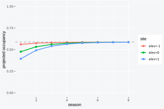

The three curves start apart, ranked by elevation, and converge on the dashed equilibrium line within a few seasons because the rates that drive them are shared. The initial spread is the covariate effect on first-season occupancy; the convergence is the dynamics washing the initial condition out. A site’s elevation buys it a head start or a deficit that the transition rates erode season by season, which is the practical reason first-season covariates matter most for short surveys and least for long ones.

To carry the full posterior uncertainty into the projection rather than the modal rates, iterate the recursion per draw as the trajectory band did, starting each draw’s curve from that draw’s $\psi_1$ at the design. The point projection above is the fast read; the per-draw version is the one to report when the horizon is long enough that the rate uncertainty compounds into a wide band by the end. Prediction here is for the occupancy side of the model; the detection probability at a new design comes from the detection arm through tobs_marginal_effect(fit, ..., process = "detection"), the same accessor the single-season vignette uses.

Comparing models

WAIC earns its keep in comparison. A single value is uninterpretable on its own; what carries meaning is the difference between two models fit to the same data. The natural comparison for a dynamic model is the dynamic fit against the structure that drops the transitions, a model that holds occupancy constant across seasons and so cannot represent colonisation or extinction. The covariate-on-colonisation fit from earlier and the constant-rate fit give a second comparison: whether the data support letting a rate vary. Fit a simpler model and read the scores side by side; the lower WAIC is the better predictor of the histories you have.

fit_cov_e <- tobs(
  ~ 1, data = dat_cov, family = dyn_occu(), detection = ~ 1, y = sim$y,
  colonization = ~ connectivity, extinction = ~ connectivity,
  method = "laplace", control = list(verbose = FALSE)
)

waic_tab <- data.frame(
  model  = c("constant rates", "connectivity on colonisation",
             "connectivity on both rates"),
  waic   = c(waic(fit)$estimates["waic", "Estimate"], waic(fit_cov)$estimates["waic", "Estimate"],
             waic(fit_cov_e)$estimates["waic", "Estimate"]),
  p_waic = c(waic(fit)$estimates["p_waic", "Estimate"], waic(fit_cov)$estimates["p_waic", "Estimate"],
             waic(fit_cov_e)$estimates["p_waic", "Estimate"])
)
waic_tab$delta <- round(waic_tab$waic - min(waic_tab$waic), 1)
waic_tab$waic  <- round(waic_tab$waic, 1)
waic_tab$p_waic <- round(waic_tab$p_waic, 2)
waic_tab
#>                          model   waic p_waic delta
#> 1               constant rates 4828.5   4.10   0.0
#> 2 connectivity on colonisation 4830.4   5.21   1.9
#> 3   connectivity on both rates 4832.8   6.42   4.3

The constant-rate model carries the lowest WAIC here, because connectivity was drawn independently of the simulated trajectory and the covariate slots add parameters the data cannot put to work. The delta column is the gap from the best model; a drop of more than a few units is the usual rough threshold for preferring the larger model, and the covariate models miss that threshold, matching how the data were generated. On a real dataset where connectivity genuinely drove colonisation, the covariate model would carry the lower WAIC and the delta would favour it, which is the signal that the predictor is doing real work on the rate rather than fitting noise.

WAIC ranks models on predictive accuracy; it does not certify that the winner is correctly specified, and it will happily hand you the less wrong of two wrong models. Pair it with the smoothed-state and residual checks above before trusting the ranking. The comparison also guides model building one decision at a time: a covariate that belongs on colonisation should lower WAIC when added to colonization and do little when forced onto extinction, the same way a single-season covariate sorts into the occupancy or the detection arm.

Full posterior with NUTS

The Laplace fit finds the mode of the four rates and the curvature there, which is fast and accurate when the likelihood is well behaved. When you want draws from the full posterior, or when few seasons and low detection make the mode an incomplete summary, method = "nuts" runs the gradient sampler over the same model. The control names are dotted: n.iter, n.warmup, and seed.

fit_nuts <- tobs(
  ~ 1,
  data        = sim$data,
  family      = dyn_occu(),
  detection   = ~ 1,
  y           = sim$y,
  colonization = ~ 1,
  extinction = ~ 1,
  method      = "nuts",
  control     = list(n.iter = 600, n.warmup = 300, seed = 1, verbose = FALSE)
)
fit_nuts$intercepts
#> $psi1
#> psi1_(Intercept) 
#>        0.4707712 
#> 
#> $p
#> p_(Intercept) 
#>     0.5004326 
#> 
#> $gamma
#> gamma_(Intercept) 
#>         0.2972662 
#> 
#> $epsilon
#> epsilon_(Intercept) 
#>           0.2093402

The sampler returns the same four rates near their simulated values. Its $intercepts are summaries of the posterior draws rather than a single mode, so the two backends agree on the rates while the sampler additionally reports the spread the Laplace approximation collapses to its curvature. Use Laplace for the first look and for speed; reach for NUTS when the rates are weakly identified or when you need the posterior shape rather than a Gaussian summary at the mode.

The difference between the two backends matters most for the extinction rate when occupancy is high or for colonisation when occupancy is low, because the relevant transitions are then rare and the likelihood for that rate is skewed rather than bell-shaped. A Gaussian summary at the mode reports a symmetric interval that can stray below zero or above one on the probability scale once back-transformed, while the sampler traces the true skew and keeps the interval where it belongs. When the equilibrium occupancy you derive depends sensitively on a rate near its boundary, the sampler’s draws also let you propagate the rate uncertainty into the derived quantity directly, by computing the equilibrium and turnover on every draw and summarising the result, rather than plugging point estimates into the formula.

Practical guidance

Dynamic occupancy asks more of a dataset than a single-season model does, because it estimates change from repeated snapshots. A few rules of thumb keep the rates identifiable.

• Use at least three seasons, and prefer five or more. Two seasons give a single transition step, which estimates one blended change but cannot separate colonisation from extinction cleanly. Three seasons give two steps and make the two rates jointly estimable; five or more seasons let the rates and the equilibrium be read with usable precision. The simulation here uses six.

• Keep at least three visits per season, more when detection is low. Within a season the model separates a true absence from a missed detection using the repeat visits, exactly as in the single-season case. With one visit per season detection and occupancy are confounded; with three or four visits and detection above about 0.3 the season-level state is well resolved. Below that detection level, add visits or move to NUTS.

• Watch the sites-times-seasons budget. The transition rates are estimated from the count of sites that change state between consecutive seasons. A few dozen sites over three seasons leaves few such transitions and wide intervals on $\gamma$ and $\epsilon$; a couple of hundred sites over five or more seasons, as here, gives hundreds of transition opportunities and tight rates. If the realised occupancy is near zero or near one, the relevant transitions become rare even at large site counts, so a mid-range occupancy is the easiest regime.

• Read the derived quantities, not just the rates. Equilibrium occupancy $\gamma / (\gamma + \epsilon)$ and turnover are usually the ecological targets, and they are smooth functions of the two rates that summarise the metapopulation better than either rate alone. A small change in $\epsilon$ near zero moves the equilibrium a long way, so report the equilibrium with the uncertainty that flows from the rate intervals rather than from a point plug-in.

• Check prior sensitivity when transitions are rare. The rates carry weakly informative priors on the logit scale, which barely move a rate that the data pin but pull a rate estimated from a handful of transitions toward its prior mean. When realised occupancy sits near zero or one, refit with the rate’s prior loosened and tightened and watch whether the posterior moves with it; a rate that tracks its prior is a rate the data did not inform, and reporting it as an estimate overstates what the survey saw. The cross-engine check below catches the same problem from the likelihood side.

• When not to fit it. If you have a single season, fit occu(); there is no transition to estimate. If you have many seasons but the species never changes state, the rates collapse to zero or one and the dynamic structure adds parameters that the data cannot inform, so a static model per season is more honest. And if seasons are so far apart that the Markov assumption fails, with several unobserved transitions folded into each observed step, the colonisation and extinction you estimate describe the observation interval rather than the biological process.

The choices above collapse into a short decision table, read top to bottom: the first row whose condition your design meets points to the model that matches what the data can actually estimate.

Your design	Fit this	Why
One season	occu()	no transition to estimate
Two seasons	occu() per season, or dyn_occu() with caution	one transition step blends colonisation and extinction
Three or more seasons, state changes	dyn_occu()	rates jointly estimable, equilibrium readable
Many seasons, state never changes	static occu() per season	rates degenerate to 0/1, dynamic params uninformed
Seasons far apart, Markov broken	dyn_occu() reporting interval-scale rates	rates describe the observation gap, not the biology

The reliable test underneath the table is the cross-engine check: fit under Laplace and under NUTS and compare the rates. When the deterministic mode and the sampled posterior agree, the design supports the model and the cheap fit is faithful; when they pull apart, the transitions are too rare to pin and only the sampler, or a longer survey, will settle the rates.

Where to go next

• Single-season occupancy, detection, and the latent state: vignette("occupancy").

• Many species surveyed at once: vignette("community-models").

• Combining detection histories from several sources: vignette("integrated-occupancy").

• Posterior-predictive checks, WAIC, and residual diagnostics: vignette("diagnostics").