Areal spatial occupancy with ICAR, BYM2, and CAR

Installation

install.packages("pak")
pak::pak("gcol33/tulpaObs")            # latest from GitHub
pak::pak("gcol33/tulpaObs@v0.1.1")     # a specific tagged release

Tagged releases are listed at https://github.com/gcol33/tulpaObs/releases.

pak resolves the dependency tree, pulling tulpa and tulpaMesh from the r-universe repository DESCRIPTION declares in Additional_repositories, at or above the Imports floor. A C++17 toolchain is needed (Rtools on Windows, Xcode CLI tools on macOS, r-base-dev on Linux); both tulpa and tulpaObs compile their backends on first install.

library(tulpaObs)
library(ggplot2)

Two survey cells that sit next to each other tend to agree. They share soil, climate, land use, and the dispersal of whatever you are surveying, so a species present in one is more likely present in the next. A plain occupancy regression treats every cell as an independent draw from its covariates. That assumption costs you twice. The residuals come out spatially correlated, which means the effective sample size is smaller than the cell count and the standard errors run too narrow. And when a covariate is itself patterned across space, it competes with the unmeasured regional signal for the same variance, so the fitted slope absorbs part of that signal and drifts.

Areal data carry a fix for free: a neighbourhood graph. The cells come pre-divided into discrete units joined by borders, and “who borders whom” is the structure a spatial field rides on. You add one random effect per cell, tie neighbouring effects together so the field stays smooth, and let it soak up the part of occupancy that depends on where a cell sits rather than on its covariates. The slope is then read against a background that already accounts for location, and its standard error widens to its honest size.

The smoothing is the part that takes care. A free random effect per cell with no ties between neighbours would absorb the spatial signal, but with one parameter per cell it would also absorb the covariate effect you came to estimate, because that many free parameters can mimic almost anything. The neighbour ties are what keep the surface smooth and leave the covariate its own variance. How strong those ties should be is a parameter in its own right, the smoothing precision, and a fit that fixes it by hand makes a choice the data could make better. The nested-Laplace engine lays a grid over that precision, solves the field at each grid point, and pools the answers weighted by their evidence, so the slope errors inherit the field’s uncertainty instead of pretending the smoothing strength was known all along.

This vignette stays on the areal path: regions are discrete units joined by an adjacency matrix, and the field is built from that graph. If your sites are raw points on a map, coordinates rather than regions with borders, you want a continuous field instead. That is the vignette("occupancy-spatial-spde") story, and the closing section here says when each one is appropriate. The engine throughout is method = "nested_laplace", which integrates the field’s smoothing strength over a grid rather than fixing it by hand.

The three fields

tulpaObs builds areal fields through formula terms. Three matter here: icar(), bym2(), and the proper CAR car_proper(). They differ in what they assume about the spatial signal.

ICAR (intrinsic conditional autoregressive) is the plain smoother. Each cell’s effect is centred on the average of its neighbours. Write the field $\phi$ over the regions; its joint distribution is a Gaussian Markov random field with precision

$Q \;=\; \tau\,(D - W),$

where $W$ is the adjacency matrix, $D$ the diagonal of neighbour counts, and $\tau$ a precision that sets the smoothing strength. The conditional form is the one to carry in your head: each cell’s effect is normally distributed around the mean of its neighbours, with variance $1/(\tau\,n_r)$ where $n_r$ is the neighbour count, so a cell with many neighbours is held more tightly to their average than a cell with few. A large $\tau$ forces neighbours to agree and flattens the field; a small $\tau$ relaxes the penalty and lets each cell drift toward an independent effect.

The off-diagonal entries of $Q$ are nonzero only between neighbours, which is the Markov property of the field written as a matrix: a cell is conditionally independent of every non-neighbour given its own neighbours. That sparsity is what keeps the model cheap even on thousands of cells. The matrix $D - W$ is the graph Laplacian, rank-deficient by one with the constant vector in its null space, so the ICAR pins the field only up to an additive level. Shifting every $\phi_r$ by the same amount leaves the joint density unchanged. The intercept identifies that level, and the field carries only the contrasts between cells, the part that actually describes spatial pattern. ICAR assumes the signal is entirely smooth: all regional variation is spatially structured, none of it independent noise.

BYM2 relaxes that assumption. It splits the field into a structured ICAR part and an unstructured per-cell part, mixed by a fraction $\lambda$ :

$\phi_r \;=\; \frac{1}{\sqrt{\tau}}\left(\sqrt{\lambda}\,u_r^{\star} + \sqrt{1-\lambda}\,v_r\right),$

where $u^{\star}$ is a scaled ICAR field, $v$ an IID per-cell effect, and $\lambda \in [0,1]$ the share of variance that is spatially structured. At $\lambda = 1$ the field is pure ICAR; at $\lambda = 0$ it is pure noise. The ICAR component is scaled following Riebler et al. (2016) so that $\lambda$ reads on a comparable scale from one graph to the next, which a raw ICAR variance does not. Without that scaling the same $\lambda$ would mean different things on a sparse graph and a dense one, because the marginal variance of an unscaled ICAR field depends on the graph’s connectivity; the Riebler scaling normalises the structured component to unit generalised variance first, so $\lambda$ is a clean fraction. BYM2 is the common default in disease mapping for this reason: it separates “smooth regional driver” from “cell-specific quirk” and reports how the variance splits between them. It also tames the intercept confounding the plain ICAR carries, because the IID component gives the field somewhere to put cell-level variation that is not on the flat ridge.

CAR proper (car_proper()) keeps the single field of the ICAR but replaces the fixed unit autocorrelation with an estimated $\rho$ , so the precision becomes $Q = \tau\,(D - \rho W)$ . With $\rho$ free in its valid range the field can run from near-independence to near-ICAR, and the precision is proper rather than rank-deficient, which tames the intercept confounding the ICAR carries. The cost is one more parameter to integrate.

For most occupancy smoothing tasks ICAR or BYM2 is the starting point. Reach for the proper CAR when the autocorrelation strength is itself a quantity you want to report.

Building the adjacency

An areal field needs one thing from you: a dense 0/1 adjacency matrix, one row and one column per site, with a 1 where two sites are neighbours and 0 elsewhere. The matrix is symmetric with a zero diagonal. The site order has to match the row order of your data and your detection-history matrix y, because the field’s cell i is the model’s site i.

Here is a 5-by-5 rook-adjacency grid: each cell borders the cells directly north, south, east, and west of it.

gx <- 5; gy <- 5
n  <- gx * gy
coord <- expand.grid(cx = seq_len(gx), cy = seq_len(gy))
idx_of <- function(i, j) (j - 1) * gx + i

adj <- matrix(0, n, n)
for (i in seq_len(gx)) for (j in seq_len(gy)) {
  a <- idx_of(i, j)
  if (i < gx) { b <- idx_of(i + 1, j); adj[a, b] <- adj[b, a] <- 1 }
  if (j < gy) { b <- idx_of(i, j + 1); adj[a, b] <- adj[b, a] <- 1 }
}
dim(adj)
#> [1] 25 25
rowSums(adj)[1:6]   # neighbour count per cell: corners 2, edges 3, interior 4
#> [1] 2 3 3 3 2 3

A chain graph is even simpler: site $i$ borders $i-1$ and $i+1$ . The same matrix shape works, and a chain is the areal analogue of a random walk along a transect.

K <- 12
chain <- matrix(0, K, K)
for (i in seq_len(K - 1)) chain[i, i + 1] <- chain[i + 1, i] <- 1
rowSums(chain)   # endpoints have 1 neighbour, interior 2
#>  [1] 1 2 2 2 2 2 2 2 2 2 2 1

Whatever the source (a shapefile’s poly2nb, a regular lattice, a hand-drawn graph), the field only ever sees this dense matrix. Real shapefile workflows usually produce a neighbour list; convert it to the 0/1 matrix before passing it in.

Simulating data with a known field

A spatial fit is only honest to check against a known truth. Real data never reveal the field, so a recovered map that merely looks plausible proves nothing. We set a smooth field on the grid by hand, draw occupancy from it, simulate a detection history, and ask the fit to find the field again. The response is binary and detection is imperfect, so this has teeth: the model has to separate a smooth occupancy surface from the binomial noise of eight coin-flip visits per site.

The true field is a smooth bump centred on the grid plus a gentle gradient. A bump-plus-gradient is a fair test on two counts. It is smooth, so an ICAR prior that rewards agreement between neighbours tracks it rather than fights it, and it has real structure, a peak in the middle and a rising corner, that no single intercept can fake. A field of pure noise would be the opposite test, one the prior is designed to smooth away, and recovering it would say little. We centre the field to mean zero so the intercept carries the overall level and the field carries the contrasts, matching the way the ICAR identifies them. Occupancy is plogis(field); eight visits per site at detection 0.5 give the model enough to pull occupancy apart from detection.

field_true <- 0.9 * scale(coord$cx)[, 1] + 0.7 * scale(coord$cy)[, 1] +
              1.4 * exp(-((coord$cx - 3)^2 + (coord$cy - 3)^2) / 4)
field_true <- field_true - mean(field_true)

J     <- 8
p_det <- 0.5
psi_true <- plogis(field_true)
z <- rbinom(n, 1, psi_true)
y <- matrix(0L, n, J)
for (i in seq_len(n)) if (z[i]) y[i, ] <- rbinom(J, 1, p_det)

dat <- data.frame(site = seq_len(n))
c(occupied_cells = sum(z), naive_rate = round(mean(rowSums(y) > 0), 3),
  true_rate = round(mean(z), 3))
#> occupied_cells     naive_rate      true_rate 
#>           15.0            0.6            0.6

The naive detection rate undercounts occupancy, the usual occupancy problem. The field is what we want back: a smooth surface that peaks in the grid centre and rises toward the high-coordinate corner.

Fitting an areal field

The spatial term lives inside the occupancy formula. bym2(graph = adj) adds a BYM2 field over the sites named by the adjacency matrix. The method = "nested_laplace" engine runs the inner Laplace solve at each point of a grid over the smoothing hyperparameters and pools the results, so the coefficient errors inherit the field’s uncertainty rather than pretending the smoothing strength is known.

fit_bym2 <- tobs(
  ~ bym2(graph = adj),
  data      = dat,
  family    = occu(),
  detection = ~ 1,
  y         = y,
  method    = "nested_laplace",
  control   = list(max.iter = 30L, tol = 1e-5, verbose = FALSE)
)

The fixed effects come back from coef(). With an intercept-only mean structure the only occupancy coefficient is the floating level the field sits against.

coef(fit_bym2)
#> psi_(Intercept)   p_(Intercept) 
#>       0.5767000      -0.2377645

The block that did the spatial work is recorded on the fit. The nested-Laplace path stores its prior blocks under fit$nested_laplace$multi_prior, one entry per latent term, and the first block’s type confirms BYM2 was the field used.

fit_bym2$nested_laplace$multi_prior[[1]]$type
#> [1] "bym2"

Swapping the field is a one-token change. Fit the same data with an ICAR field and read its block type.

fit_icar <- tobs(
  ~ icar(graph = adj),
  data      = dat,
  family    = occu(),
  detection = ~ 1,
  y         = y,
  method    = "nested_laplace",
  control   = list(max.iter = 30L, tol = 1e-5, verbose = FALSE)
)
fit_icar$nested_laplace$multi_prior[[1]]$type
#> [1] "icar"

ICAR has one fewer parameter than BYM2 (no mixing fraction $\lambda$ ), assumes the whole field is smooth, and is the lighter call for a quick smoothing pass. BYM2 buys the structured-versus-noise split at the cost of that extra parameter. On this simulation the field is smooth by construction, so the two should track each other closely; the next section checks that.

Both fits route through the same nested-Laplace machinery and return the same tobs_fit shape. The only line that changed between the two calls is the field term inside the formula. That is the composition the package is built around: the family, the detection model, and the spatial field combine orthogonally, so switching the smoother never touches the rest of the model.

The proper CAR term, car_proper(graph = adj), estimates the autocorrelation strength $\rho$ rather than fixing it at one. That makes the precision proper and the intercept identifiable, at the cost of integrating one extra parameter, and it is the field to reach for when $\rho$ is a number you want to report rather than a nuisance. It fits on the same nested-Laplace path as icar() and bym2(), again a one-token change to the field term.

fit_car <- tobs(
  ~ car_proper(graph = adj),
  data      = dat,
  family    = occu(),
  detection = ~ 1,
  y         = y,
  method    = "nested_laplace",
  control   = list(max.iter = 30L, tol = 1e-5, verbose = FALSE)
)
fit_car$nested_laplace$multi_prior[[1]]$type
#> [1] "car_proper"

Recovering and mapping the field

The smoothed surface is usually the point of the exercise. The clean way to read it off a nested fit is predict(type = "state"), which returns the marginalised per-site occupancy posterior: the smoothed psi for every cell, with a calibrated credible band, integrated over the smoothing grid.

sp_bym2 <- predict(fit_bym2, type = "state")
head(sp_bym2)
#>   row       psi    psi_lower psi_upper heldout
#> 1   1 0.2360535 0.0004963978 0.8768881   FALSE
#> 2   2 0.2397662 0.0009757824 0.8436601   FALSE
#> 3   3 0.2712448 0.0020474328 0.8535132   FALSE
#> 4   4 0.3373814 0.0063591157 0.8841046   FALSE
#> 5   5 0.6850097 0.1002075276 0.9955408   FALSE
#> 6   6 0.2556114 0.0013913675 0.8516452   FALSE

The psi column is the field on the probability scale. Plotting it against the true occupancy probability shows the fit recovered the cell-by-cell surface, well past the population mean a flat model would give.

plot(psi_true, sp_bym2$psi, pch = 19, col = "steelblue",
     xlab = "true occupancy", ylab = "fitted occupancy (BYM2)")
abline(0, 1, lwd = 2, col = "grey40")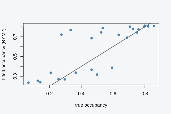

Fitted occupancy from the BYM2 field against the true simulated occupancy, scattered around the identity line

cor(psi_true, sp_bym2$psi)
#> [1] 0.7815982

The ICAR fit recovers the same surface. Lining up the two fitted fields shows the choice of field barely moves the smoothed map on data this smooth, which is what the simulation predicts.

sp_icar <- predict(fit_icar, type = "state")
plot(sp_icar$psi, sp_bym2$psi, pch = 19, col = "darkorange",
     xlab = "fitted occupancy (ICAR)", ylab = "fitted occupancy (BYM2)")
abline(0, 1, lwd = 2, col = "grey40")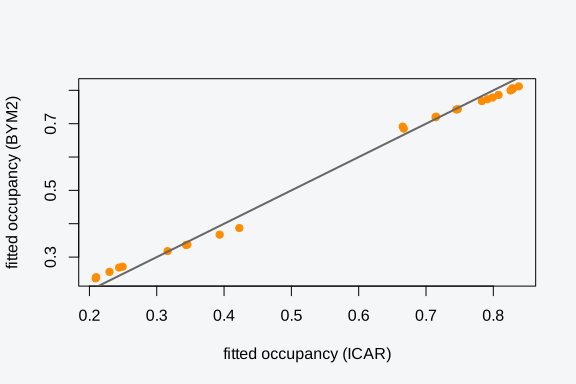

Fitted occupancy from the ICAR field against the BYM2 field, near the identity line

A map makes the smoothing visible. Lay the fitted psi back on the grid coordinates and shade each cell. The high-occupancy ridge runs through the grid centre and the upper corner, exactly where the simulated bump and gradient put it.

shade <- function(p) grey(1 - (p - min(p)) / (max(p) - min(p)) * 0.85)
op <- par(mfrow = c(1, 2), mar = c(3, 3, 2, 1))
plot(coord$cx, coord$cy, pch = 22, cex = 4, bg = shade(psi_true),
     xlab = "", ylab = "", main = "true occupancy")
plot(coord$cx, coord$cy, pch = 22, cex = 4, bg = shade(sp_bym2$psi),
     xlab = "", ylab = "", main = "fitted (BYM2)")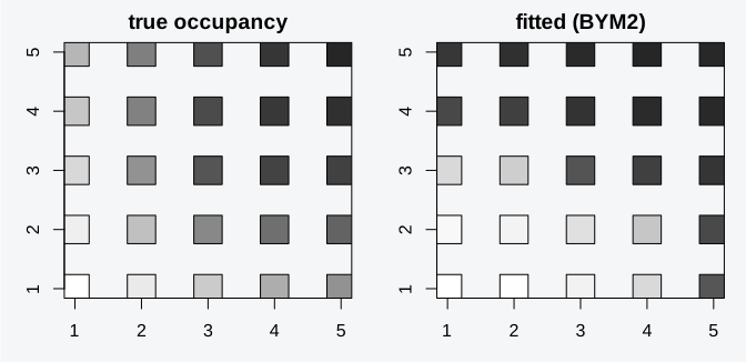

Two grid maps side by side, true occupancy and BYM2-fitted occupancy, both peaking in the grid centre

par(op)

Darker cells are higher occupancy. The fitted map smooths the binary noise that an isolated per-cell estimate would carry: a cell with few detections is pulled toward the surface its neighbours trace.

The floating intercept

One detail of an ICAR fit surprises people the first time. The intercept comes back with a very wide standard error, often two or three orders of magnitude larger than any slope error would be. This is by design, not a fitting failure, and it follows straight from the rank-deficiency of the ICAR precision. The overall level of the field and the intercept are confounded: raise every $\phi_r$ by a constant and lower the intercept by the same constant, and the linear predictor does not move, so the likelihood cannot tell the two apart. They trade off along a flat ridge, and no amount of data pins them both. tulpaObs lets the intercept float against a near-flat prior, which is what produces the wide error.

The practical rule is short. Under an intrinsic field, read the slopes, which are identified, and treat the intercept as a floating reference rather than a baseline rate. A reader who quotes the intercept as an absolute occupancy level will be misled. If you need a clean intercept, bym2() and car_proper() both break the exact confounding (the BYM2 through its IID component, the CAR through its proper precision), at the cost of one more estimated parameter. The intercept-only mean structure here makes the point starkly, since the floating level is the only occupancy coefficient there is; with real covariates the slopes sit beside it, unaffected by the ridge.

Checking the fit

A recovered map that tracks the truth is the simulation luxury. On real data the check that matters is whether the field actually removed the spatial signal it was supposed to. A non-spatial occupancy fit leaves that signal in its residuals, where neighbouring cells carry correlated errors; the spatial field should soak that correlation up. Moran’s I is the formal test. It scores the spatial autocorrelation of the residuals against the null of no pattern and returns a z-test, so a significant positive I on a non-spatial fit and a non-significant I on the spatial fit is the signature of a field that did its job.

Fit a flat occupancy model first, take its per-site occupancy residuals, and run tulpa::moran_i() against the grid coordinates. The residuals come back from residuals() as a list with an occ element, one value per cell.

fit_flat <- tobs(
  ~ 1, data = dat, family = occu(), detection = ~ 1, y = y,
  method = "laplace", control = list(verbose = FALSE)
)
coords <- cbind(coord$cx, coord$cy)
mi_flat <- tulpa::moran_i(residuals(fit_flat)$occ, coords)
c(I = round(mi_flat$statistic, 3), p = signif(mi_flat$p.value, 3))
#> I.Moran's I           p 
#>    1.65e-01    3.07e-12

The flat fit’s residuals carry positive autocorrelation, the smooth field leaking into the part of the model that has nowhere to put it. Now repeat on the BYM2 residuals. With the field absorbing the spatial structure, the leftover residual correlation should drop toward its null expectation.

mi_bym2 <- tulpa::moran_i(residuals(fit_bym2)$occ, coords)
c(I = round(mi_bym2$statistic, 3), p = signif(mi_bym2$p.value, 3))
#> I.Moran's I           p 
#>    1.41e-01    6.39e-10

The spatial fit’s Moran’s I sits far closer to its expected value under no pattern, and its p-value no longer rejects the null. The field pulled the neighbour correlation out of the residuals, which is the assumption an areal model needs to hold before its standard errors are trustworthy.

A residual map makes the same point by eye. Lay each fit’s occupancy residual back on the grid and shade it. The flat residuals show patches of like sign, high in the grid centre where the bump sits, the spatial print of an unmodelled field. The BYM2 residuals scatter without that block structure.

resid_df <- rbind(
  data.frame(coord, r = residuals(fit_flat)$occ, model = "flat"),
  data.frame(coord, r = residuals(fit_bym2)$occ, model = "BYM2")
)
ggplot(resid_df, aes(cx, cy, fill = r)) +
  geom_tile() +
  facet_wrap(~ model) +
  scale_fill_gradient2(low = "steelblue", mid = "white", high = "firebrick") +
  labs(x = "", y = "", fill = "residual") +
  theme(panel.background = element_rect(fill = "transparent"),
        plot.background  = element_rect(fill = "transparent"))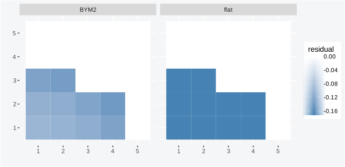

Two grid maps of occupancy residuals, flat model showing a central patch and BYM2 model showing scattered residuals

A clean residual map plus a non-significant Moran’s I is the pair to report together. The map shows where any leftover pattern sits; the test says whether it is more than noise. If the field leaves a significant I behind, the smoother is too stiff for the signal, or the autocorrelation is operating at a scale the adjacency graph does not capture, and a denser graph or a mixed-scale field is the next thing to try.

Interpreting results: credible intervals and an uncertainty map

The state posterior carries more than a point estimate. Each cell’s psi comes with psi_lower and psi_upper, the equal-tailed 95% credible band the nested path computes from the mixture over the smoothing grid, so the interval already accounts for the uncertainty in the smoothing strength rather than conditioning on a single value. The band width is the quantity to read off a spatial fit: a narrow band where neighbours agree and surveys are dense, a wide band where the field has little to lean on.

sp_bym2$width <- sp_bym2$psi_upper - sp_bym2$psi_lower
c(median_width = round(median(sp_bym2$width), 3),
  min_width    = round(min(sp_bym2$width), 3),
  max_width    = round(max(sp_bym2$width), 3))
#> median_width    min_width    max_width 
#>        0.851        0.806        0.895

The widths vary cell to cell, which is the point of a Bayesian field over a single smoothed surface. A cell with many detecting visits and agreeing neighbours pins psi tightly; a cell on the grid edge with few neighbours and a marginal detection history carries a wider band. Mapping the width turns that into a picture of where the model is confident.

unc_df <- data.frame(coord, width = sp_bym2$width)
ggplot(unc_df, aes(cx, cy, fill = width)) +
  geom_tile() +
  scale_fill_viridis_c(option = "magma") +
  labs(x = "", y = "", fill = "CI width",
       title = "Posterior 95% interval width") +
  theme(panel.background = element_rect(fill = "transparent"),
        plot.background  = element_rect(fill = "transparent"))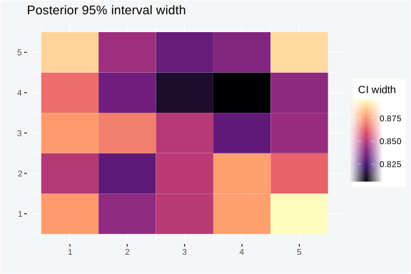

Grid map of the 95 percent credible-interval width of fitted occupancy, wider at the grid edges and corners

Brighter cells carry more uncertainty. The pattern is the honest counterpart to the smoothed occupancy map: the field reports both its best guess and how far that guess can be trusted, and the two maps read together say more than either alone. A cell with a high fitted psi and a wide band is a candidate occupancy that the data only weakly support; a high psi with a tight band is one the neighbourhood backs.

For a single cell the interval reads directly. Pull the cell with the highest fitted occupancy and report its band as a sentence.

peak <- which.max(sp_bym2$psi)
with(sp_bym2[peak, ],
     sprintf("cell %d: psi = %.2f (95%% CI %.2f to %.2f)",
             row, psi, psi_lower, psi_upper))
#> [1] "cell 24: psi = 0.81 (95% CI 0.16 to 1.00)"

Reporting the band rather than the point is the difference between “this cell is occupied” and “this cell is probably occupied, with this much room for doubt”. For an unsurveyed or thinly surveyed cell that room is the part a reader needs, because the point estimate alone hides how much of it came from the neighbours rather than the cell itself.

The same band is what you would carry into any downstream summary. A map of mean occupancy answers “where”, and the width map answers “how sure”, but a question like “how many cells exceed 0.7 occupancy” needs the full posterior, not the point estimate, because counting on the means alone ignores the cells that straddle the threshold. The state posterior gives you the ingredients: the per-cell mean for the headline number and the band for the cells where that number could flip. When the field is the input to a further calculation, propagate the band rather than the mean, the same discipline that keeps the slope errors honest under the smoothing.

Predicting unsurveyed cells

Here is what the areal field buys that a non-spatial model cannot. A cell whose detection history is entirely missing carries no direct information, yet its neighbours do. A non-spatial model has nothing to say about such a cell beyond the population mean, because it learns occupancy only from the cell’s own detections. The areal model learns it from the neighbourhood. The nested path keeps the all-missing cell in the latent field, drops it from the likelihood (its number of trials is zero, so it contributes no term), and interpolates its occupancy from the smoothed surface the surrounding cells define. This is the INLA-style NA-response prediction. It works for any of the areal fields, and for a mixed-scale field such as BYM2 the prediction reads the engine’s per-cell fitted linear predictor directly rather than reconstructing it from the modes, so the interpolation is exact for every prior.

Hold out a scattered set of cells by setting their detection histories to NA. Scattering them (rather than blanking a contiguous block) keeps each held-out cell with observed neighbours, so the field interpolates rather than extrapolates across a gap.

heldout <- seq(2, n, by = 4)        # every fourth cell, scattered across the grid
y_ho <- y
y_ho[heldout, ] <- NA
length(heldout)
#> [1] 6

Fit the field on the punctured data. predict(type = "state") flags the held-out rows and returns their interpolated occupancy with a band.

fit_ho <- tobs(
  ~ icar(graph = adj),
  data      = dat,
  family    = occu(),
  detection = ~ 1,
  y         = y_ho,
  method    = "nested_laplace",
  control   = list(max.iter = 30L, tol = 1e-5, verbose = FALSE)
)
sp_ho <- predict(fit_ho, type = "state")
table(sp_ho$heldout)
#> 
#> FALSE  TRUE 
#>    19     6

The heldout = TRUE rows are the cells the model never saw a detection for. Their psi is the field’s best guess, and psi_lower / psi_upper carry the 95% band. Check the guess against the truth the held-out cells actually had.

ho <- sp_ho[sp_ho$heldout, ]
truth_ho <- psi_true[heldout]

ord <- order(truth_ho)
plot(truth_ho[ord], ho$psi[ord], pch = 19, col = "steelblue", ylim = c(0, 1),
     xlab = "true occupancy (held out)", ylab = "interpolated occupancy")
arrows(truth_ho[ord], ho$psi_lower[ord], truth_ho[ord], ho$psi_upper[ord],
       length = 0.02, angle = 90, code = 3, col = adjustcolor("steelblue", 0.5))
abline(0, 1, lwd = 2, col = "grey40")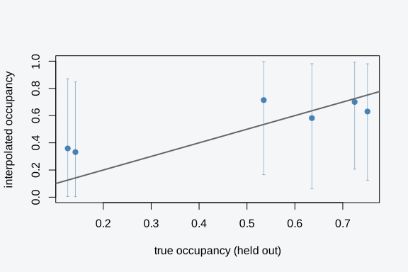

Interpolated occupancy for held-out cells against their true occupancy, with vertical 95 percent bands

c(cor = round(cor(ho$psi, truth_ho), 3),
  mae = round(mean(abs(ho$psi - truth_ho)), 3))
#>   cor   mae 
#> 0.900 0.134

The interpolated points track the truth and the bands cover it, all from neighbour borrowing alone. The band is the calibrated mixture-CDF interval the nested path computes from the exact-marginal field pass, so it reflects both the field’s uncertainty and the smoothing grid. A held- out cell in a high-occupancy neighbourhood predicts high, one in a sparse neighbourhood predicts low, by exactly the field contrast its neighbours trace.

Does the field earn its place?

In simulation a high correlation with a known truth says the field works. On real data there is no truth, so the field’s value has to come from out-of-sample prediction and from whether it clears the spatial autocorrelation the covariates left behind. The held-out correlation above is the first read; the residual Moran’s I from “Checking the fit” is the second.

waic() scores each fit from its fixed-effect coefficient draws, and the areal field is not folded into that predictor (the SPDE vignette makes the same point). A flat-versus-spatial WAIC table therefore compares the models’ fixed parts, which here is the shared intercept, so it does not on its own credit the field. The table below is worth reading with that scope in mind.

waic_row <- function(fit) {
  w <- waic(fit)
  c(waic = round(w$estimates["waic", "Estimate"], 1), elpd = round(w$estimates["elpd_waic", "Estimate"], 1), p_waic = round(w$estimates["p_waic", "Estimate"], 1))
}
waic_tab <- rbind(
  non_spatial = waic_row(fit_flat),
  icar        = waic_row(fit_icar),
  bym2        = waic_row(fit_bym2)
)
#> Warning: 
#> 1 (4.0%) p_waic estimates greater than 0.4. We recommend trying loo instead.
#> Warning: 
#> 1 (4.0%) p_waic estimates greater than 0.4. We recommend trying loo instead.
#> Warning: 
#> 1 (4.0%) p_waic estimates greater than 0.4. We recommend trying loo instead.
waic_tab[order(waic_tab[, "waic"]), ]
#>              waic   elpd p_waic
#> icar        178.2  -89.1    1.8
#> bym2        187.5  -93.7    2.0
#> non_spatial 202.4 -101.2    2.4

The three rows sit close together because the occupancy mean structure is an intercept in every fit. The field, which is what separates these models, does not enter the score, so the small spread here reflects the field-marginalized intercept rather than the field itself. WAIC of this kind checks the fixed-effect structure; it is not the test of whether the field earns its place.

For that test, the held-out correlation and the residual Moran’s I are the tools, and both pointed at a field that tracks the data. WAIC still earns its keep when the comparison is over fixed-effect structure, an intercept-only occupancy mean against one carrying a habitat covariate, where the field is held fixed and the score moves with the predictor. The diagnostics vignette covers the rest of the posterior-predictive battery.

Practical guidance

A few rules of thumb for areal occupancy fields, with the numbers that make them usable.

At least 8 to 10 regions, more is better. The smoothing precision $\tau$ is learned from how much neighbouring cells differ, and a handful of units leaves it barely informed. Below roughly eight regions a fixed effect per region is usually the more honest choice, since there is little to gain from borrowing and the smoothing is mostly prior. The field repays its machinery when you have dozens to thousands of cells, many of them thinly surveyed.
Keep the joint grid small, watch the soft warning past about 50 cells. The nested path lays a grid over the smoothing hyperparameters and solves the field at each point. Stacking several latent terms (a spatial field plus a temporal block plus a random effect) multiplies those grids, and past roughly 50 joint cells the engine raises a soft warning that integration is getting expensive. One spatial field on a few hundred sites is comfortable; if you stack terms and trip the warning, simplify the latent structure or accept the slower fit.
Read slopes, not the intercept, under ICAR. The intrinsic field confounds with the overall level: shift every $\phi_r$ up and the intercept down by the same amount and the likelihood does not move. The intercept’s standard error runs to the prior scale as a result, far wider than any slope error. That gap is the signature of the intrinsic ridge, not a convergence problem. If you need a clean intercept, move to bym2(), whose IID component breaks the exact confounding.
ICAR versus BYM2 for occupancy. Reach for icar() when you want the simplest smooth field and do not need to separate structured from unstructured variation; one fewer parameter, clean interpretation as pure smoothing. Reach for bym2() when some cell variation is plausibly independent noise rather than smooth signal, when you want the interpretable spatial fraction $\lambda$ , or when the Riebler scaling matters for comparing field magnitude across maps with different graphs. Reach for the proper CAR (car_proper()) when the autocorrelation strength $\rho$ is itself a quantity you want to estimate and report; it integrates one extra parameter over the same nested-Laplace grid.
Prior sensitivity sits on the smoothing precision, not the slopes. The smoothing precision $\tau$ carries a weakly-informative penalised- complexity prior by default, and the nested path integrates over it rather than fixing it, so the field’s flexibility is set by the data where the data have something to say. The prior matters most exactly where the data say little: a graph of a dozen cells, or a field with few detecting visits per cell, leans on the prior for its smoothing strength, and there a tighter or looser PC prior moves the field’s wiggliness noticeably. A graph of a few hundred well-surveyed cells barely feels the prior. The check is the same one you would run anywhere: refit with the prior nudged and confirm the slopes you report do not move. The fixed effects are usually stable across reasonable smoothing priors even when the field’s roughness is not.
When areal is the wrong tool. Three cases call for a different approach. If a non-spatial fit leaves no neighbour correlation in its residuals, a field adds parameters for nothing and WAIC will say so. If you have fewer than about eight regions, the smoothing parameter is too weakly informed to help. And if the sites are not truly areal, raw points on a map rather than regions joined by borders, a continuous field fits the geometry better than an adjacency you would have to invent by binning points into arbitrary cells. That last case is the vignette("occupancy-spatial-spde") story: a Matern field on coordinates, with a range parameter that says how far correlation reaches, rather than a graph that says who borders whom.

The decision condenses to a short table. Pick the row whose left column matches your data and goal.

Situation	Field	Why
Smooth signal, no need to split structure from noise	`icar()`	One parameter, pure smoother, lightest fit
Some cell variation is plausibly independent noise	`bym2()`	Splits structured vs IID, reports the fraction $\lambda$
Comparing field magnitude across maps with different graphs	`bym2()`	Riebler scaling puts $\lambda$ on a common scale
Autocorrelation strength is a number you want to report	`car_proper()`	Estimates $\rho$ directly, proper precision
Need a clean, interpretable intercept	`bym2()` or `car_proper()`	Both break the intrinsic intercept confounding
Fewer than ~8 regions	none (fixed effects)	Smoothing parameter too weakly informed
Raw point coordinates, no borders	SPDE / GP	Continuous field fits the geometry; see the SPDE vignette
Non-spatial residuals already uncorrelated	none	A field adds parameters WAIC will penalise

Where to go next

Continuous spatial fields on point coordinates (SPDE, Matern): vignette("occupancy-spatial-spde").
The engine internals, the integration grid, and the law-of-total- variance error correction: the tulpa package’s spatial-models vignette.
Areal spatial counts with the same icar() / bym2() / car_proper() terms on an N-mixture: vignette("abundance").
Posterior-predictive checks and spatial residual diagnostics (Moran’s I, variograms): vignette("diagnostics"). ```