Occupancy with a continuous SPDE spatial field

Installation

install.packages("pak")
pak::pak("gcol33/tulpaObs")            # latest from GitHub
pak::pak("gcol33/tulpaObs@v0.1.1")     # a specific tagged release

Tagged releases are listed at https://github.com/gcol33/tulpaObs/releases.

pak resolves the dependency tree, pulling tulpa and tulpaMesh from the r-universe repository DESCRIPTION declares in Additional_repositories, at or above the Imports floor. A C++17 toolchain is needed (Rtools on Windows, Xcode CLI tools on macOS, r-base-dev on Linux); both tulpa and tulpaObs compile their backends on first install.

library(tulpaObs)
library(ggplot2)

Introduction

Occupancy data are usually spatially structured: nearby sites share habitat and species pressures that the row-wise covariates can’t fully capture. The Matern field via the SPDE approach (Lindgren, Rue & Lindstrom, 2011) gives a continuous spatial random effect with an interpretable range and marginal SD, and an spde() term in the formula wires it through tulpaObs’s Laplace EM engine.

The choice between a continuous field and an areal field follows from what your sites are. Areal data arrive pre-divided into regions joined by borders: census tracts, grid cells, administrative units. The neighbour graph is given, and an ICAR or BYM2 field rides on “who borders whom”. Point data arrive as raw coordinates, transects walked, traps set, plots placed on a continuous landscape, with no natural partition into cells. Forcing those points into an adjacency means binning them into arbitrary squares first, and the answer then depends on the grid you drew. A continuous field skips that step. It places a Matern process directly on the coordinates, so two sites 200 m apart are correlated more strongly than two sites 2 km apart, and the strength is set by a range parameter rather than a hand-drawn graph. That is the case this vignette covers: occupancy surveyed at scattered locations, with a smooth spatial signal in psi that no covariate measures.

Ignoring that signal costs twice. The occupancy residuals come out spatially correlated, which means the effective sample size is smaller than the site count and the standard errors run too narrow. And when an occupancy covariate is itself patterned across space, it competes with the unmeasured spatial signal for the same variance, so the fitted slope absorbs part of that signal and drifts away from its true value. A spatial field gives the location-driven part of occupancy a place to live, separate from the covariate effects, so the slope is read against a background that already accounts for where a site sits. The field also turns the missing-data problem around: a location with no survey borrows occupancy from its neighbours through the smooth surface, which a covariate-only model cannot do at all.

This vignette simulates an occupancy dataset with a known smooth spatial signal, fits a non-spatial model and an SPDE model, and compares them on parameter recovery and the latent state. It then predicts the field at unsurveyed coordinates, checks the residuals for leftover spatial structure, and closes with the rules of thumb that decide when the field is worth fitting.

The model

The single-season occupancy model has two layers. A latent presence state $z_i \in \{0, 1\}$ at site $i$ is Bernoulli with occupancy probability $\psi_i$, and the detection history $y_{ij}$ over $J$ visits is Bernoulli with detection probability $p_i$ when $z_i = 1$ and zero otherwise. The occupancy logit carries the spatial field:

$$\operatorname{logit}(\psi_i) = \mathbf{x}_i^\top \boldsymbol\beta + u(\mathbf{s}_i), \qquad \operatorname{logit}(p_i) = \mathbf{w}_i^\top \boldsymbol\alpha .$$

Here $\mathbf{x}_i$ is the occupancy covariate row at site $i$, $\boldsymbol\beta$ its coefficients, $\mathbf{w}_i$ and $\boldsymbol\alpha$ the detection covariates and their coefficients, and $\mathbf{s}_i$ the spatial coordinates of site $i$. The term $u(\mathbf{s})$ is a continuous Gaussian random field: a smooth surface defined everywhere on the study area, evaluated at each site’s coordinates.

The field is a Matern process. Its covariance between two points depends only on the distance $d$ between them,

$$\operatorname{Cov}\bigl(u(\mathbf{s}), u(\mathbf{s}')\bigr) = \sigma^2 \, \frac{2^{1-\nu}}{\Gamma(\nu)} (\kappa d)^\nu K_\nu(\kappa d),$$

with marginal standard deviation $\sigma$, smoothness $\nu$, and inverse range $\kappa$; $K_\nu$ is the modified Bessel function of the second kind. The range $\rho = \sqrt{8\nu}/\kappa$ is the distance at which correlation drops to about 0.1, the practical reach of the field. Lindgren, Rue & Lindstrom (2011) show this Matern field is the stationary solution of a stochastic partial differential equation, and that solving the SPDE on a triangular mesh gives a Gaussian Markov random field: a discrete approximation $u(\mathbf{s}) \approx \sum_k A_{ik} u_k$ where $u_k$ are values at the mesh nodes and $A$ is a sparse projection matrix that interpolates them to the site. The node values $u_k$ have a sparse precision matrix built from the mesh geometry and $(\kappa, \sigma)$, which is what keeps the field cheap even on thousands of sites. The spde() term builds the mesh, the projection $A$, and the precision at the prior modes of $\rho$ and $\sigma$.

The smoothness $\nu$ is fixed rather than estimated, and the engine defaults to $\nu = 1$, which makes the field once-differentiable and is the common choice for ecological surfaces; it is rarely identifiable from data the way $\rho$ and $\sigma$ are, so fixing it costs little. The two hyperparameters that do carry information, the range $\rho$ and the marginal SD $\sigma$, are set through PC priors (Simpson et al., 2017). A PC prior is given as a tail statement: for the range, $P(\rho < \rho_0) = p$, naming a small reference range $\rho_0$ and the probability the true range falls below it; for the SD, $P(\sigma > \sigma_0) = p$. That form penalises the field toward the simpler no-field model (infinite range, zero SD) and pulls back only as far as the data demand, which is why a range or SD prior set at a sensible scale rarely over-fits. The field enters the occupancy logit with mean zero, so the intercept $\beta_0$ carries the overall occupancy level and the field carries only the contrasts between locations, matching the way the data identify the two.

Simulating data

A spatial fit is only honest against a known truth, because a recovered map that merely looks plausible proves nothing. We set a smooth field on the unit square by hand, draw occupancy from it, simulate a detection history with imperfect detection, and ask the fit to find the field again. The field is $0.8\cos(3x)\sin(3y)$ on the logit scale: a smooth ripple with an amplitude of about 0.8, peaks and troughs at opposite corners, and real structure that no single intercept can fake. The amplitude matters. At 0.8 on the logit scale the field moves occupancy from roughly 0.3 to 0.7 across the square, enough signal for the model to separate from binomial noise, and small enough that detection still has teeth.

n_sites <- 400
J <- 8
coords <- cbind(runif(n_sites), runif(n_sites))

# A smooth spatial signal: amplitude ~0.8 on the logit scale
u_true <- 0.8 * cos(3 * coords[, 1]) * sin(3 * coords[, 2])

x_cov   <- rnorm(n_sites)
det_cov <- rnorm(n_sites)
beta_occ_true <- c(-0.5, 0.7)
beta_det_true <- c(-0.3, 0.4)

eta_occ <- beta_occ_true[1] + beta_occ_true[2] * x_cov + u_true
psi <- plogis(eta_occ)
z <- rbinom(n_sites, 1, psi)

eta_det <- beta_det_true[1] + beta_det_true[2] * det_cov
p <- plogis(eta_det)

y <- matrix(0L, n_sites, J)
for (i in seq_len(n_sites)) {
  if (z[i] == 1L) y[i, ] <- rbinom(J, 1, p[i])
}

dat <- data.frame(occ_cov = x_cov, det_cov = det_cov,
                  lon = coords[, 1], lat = coords[, 2])
c(true_occupancy_rate = mean(z),
  naive_any_detection = mean(rowSums(y) > 0))
#> true_occupancy_rate naive_any_detection 
#>                0.35                0.34

The naive any-detection rate is biased low by (1 - p)^J at each occupied site; a proper occupancy fit should correct that bias, and a spatial fit should additionally recover the smooth field that drives the site-to-site variation in psi. The data.frame keeps the coordinate columns lon and lat alongside the covariates, because the spde() term resolves those columns from data the way mgcv resolves s(lon, lat). There is no separate spatial-field simulator in the package; simulate_occu() draws covariate-only occupancy, so a known continuous field is set by hand as above. A map of the truth shows what the fit has to recover.

truth_df <- data.frame(lon = coords[, 1], lat = coords[, 2], u = u_true)
ggplot(truth_df, aes(lon, lat, colour = u)) +
  geom_point(size = 2) +
  scale_colour_viridis_c() +
  labs(title = "True latent field u(s)", colour = "u") +
  theme(panel.background = element_rect(fill = "transparent"),
        plot.background  = element_rect(fill = "transparent"))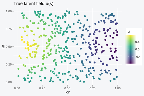

The ripple is the part we want back: a smooth surface that the non-spatial fit has no place to put, so it will leak into the intercept and the residuals.

Two design choices in the simulation make the test fair. Eight visits per site at moderate detection give the model enough replication to pull occupancy apart from detection; with one or two visits the latent state is barely identified and any field would inherit that ambiguity rather than the spatial signal. And the sites are scattered uniformly over the square rather than clustered, so every part of the field has data nearby and the recovery measures the field, not the sampling design. A clustered design would leave large gaps where the field is pure prior, which is a real situation but a different question from whether the estimator works. The covariate occ_cov is independent of the coordinates by construction, so the simulation isolates the field: any shift in the occupancy slope between the non-spatial and SPDE fits comes from the field absorbing residual variance, not from confounding between the covariate and the spatial signal. On real data those two are usually entangled, which is the harder case the field is built for, but the clean simulation is the right place to confirm the machinery first.

Fitting the model

The spatial field is written directly into the occupancy formula as an spde() term, the way mgcv writes s(lon, lat). spde() builds a triangular mesh over the observation coordinates (via tulpaMesh) and constructs the SPDE precision at the prior modes of prior.range and prior.sigma. The mesh covers the data extent plus a small buffer; max.edge = c(inner, outer) controls the spacing inside and outside the data. The coordinate columns (lon, lat) are taken from data. We fit a non-spatial model first as the baseline, then the SPDE model, so the two are directly comparable.

fit_ns <- tobs(
  formula   = ~ occ_cov,
  data      = dat,
  family    = occu(),
  detection = ~ det_cov,
  y         = y,
  method    = "laplace",
  control   = list(verbose = FALSE)
)
round(fit_ns$means, 3)
#> psi_(Intercept)     psi_occ_cov   p_(Intercept)       p_det_cov 
#>          -0.644           0.575          -0.237           0.389

The SPDE call adds one term to the occupancy formula and changes nothing else. The prior.range = c(0.3, 0.5) is a PC prior on the range: the first number is the median range guess (0.3 of the unit square), the second the probability the range is below it. prior.sigma = c(0.7, 0.5) is the matching prior on the marginal SD. max.edge = c(0.3, 0.6) sets the mesh spacing inside and outside the data; nu = 1 fixes the Matern smoothness.

fit_sp <- tobs(
  formula   = ~ occ_cov + spde(lon, lat,
                               max.edge    = c(0.3, 0.6),
                               nu          = 1,
                               prior.range = c(0.3, 0.5),
                               prior.sigma = c(0.7, 0.5)),
  data      = dat,
  family    = occu(),
  detection = ~ det_cov,
  y         = y,
  method    = "laplace",
  control   = list(verbose = FALSE)
)
round(fit_sp$means, 3)
#> psi_(Intercept)     psi_occ_cov   p_(Intercept)       p_det_cov 
#>          -0.751           0.599          -0.233           0.386

The fixed-effect coefficients come back through coef(), named by process: psi for occupancy, p for detection. The standard errors and credible intervals are in summary(), which reports the estimate, standard error, and the lower and upper credible bounds for every fixed effect.

coef(fit_sp)
#> psi_(Intercept)     psi_occ_cov   p_(Intercept)       p_det_cov 
#>      -0.7512681       0.5991743      -0.2333621       0.3860616
round(summary(fit_sp), 3)
#>                 estimate std.error  2.5 % 97.5 %
#> psi_(Intercept)   -0.751     0.118 -0.983 -0.519
#> psi_occ_cov        0.599     0.124  0.356  0.842
#> p_(Intercept)     -0.233     0.066 -0.363 -0.104
#> p_det_cov          0.386     0.066  0.256  0.516

The fitted SPDE field itself is stored on the fit as spatial_field, a length-n_mesh numeric vector at the mesh nodes, the posterior mode of the node values $u_k$. The mesh that carries it lives under fit_sp$spatial$tulpa_spec, including the projection matrix A and the node count n_mesh.

u_hat <- fit_sp$spatial_field
mesh  <- fit_sp$spatial$tulpa_spec$mesh
c(n_mesh_nodes  = fit_sp$spatial$tulpa_spec$n_mesh,
  field_length  = length(u_hat),
  field_sd      = round(sd(u_hat), 3))
#> n_mesh_nodes field_length     field_sd 
#>      420.000      420.000        0.667

The 400 sites expand to a few hundred mesh nodes, more nodes than sites because the mesh adds a buffer of nodes around the data so the field does not distort at the edges. The field SD around 0.4 is the fitted analogue of the simulated amplitude, damped by the SPDE prior’s smoothing.

Checking the fit

The first check is recovery of the field at the sites. Project the node values to the observation locations through the spec’s A matrix and line them up against the truth. A correlation well above zero says the field found the signal; the non-spatial fit has no field at all, so its only comparison is the flat population mean.

field_at_sites <- as.numeric(fit_sp$spatial$tulpa_spec$A %*% u_hat)
corr <- cor(field_at_sites, u_true)
cat(sprintf("Correlation field-at-sites vs truth: %.3f\n", corr))
#> Correlation field-at-sites vs truth: 0.652

op <- par(mfrow = c(1, 2), mar = c(4, 4, 2, 1))
plot(u_true, field_at_sites, pch = 16, col = rgb(0, 0, 0, 0.4),
     xlab = "truth u(s)", ylab = "fitted u_hat(s)",
     main = "Field recovery at sites")
abline(0, 1, col = 2, lwd = 2)
plot(coords[, 1], coords[, 2], pch = 16, cex = 0.6,
     col = ifelse(field_at_sites > 0, "red", "blue"),
     xlab = "x", ylab = "y", main = "Fitted field sign")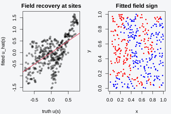

par(op)

The fitted field is regularized by the SPDE prior, so it is smoother than the truth and slightly attenuated in amplitude. The site-level correlation with the truth is well above what the non-spatial fit could achieve, where there is no field at all.

The formal check is whether any spatial structure is left in the residuals. If the field has absorbed the smooth signal, the occupancy residuals should look spatially random; leftover autocorrelation means the field missed something or the range was set wrong. check_model() runs the model diagnostics and, given the coordinates, computes Moran’s I on the occupancy residuals, the standard test for spatial autocorrelation. It also reports WAIC and a posterior predictive Bayesian p-value. Run it on both fits.

chk_ns <- check_model(fit_ns, coords = coords, n.samples = 200, plot = FALSE)
#> === tobs Model Diagnostics ===
#> 
#> Fit: laplace, 1000 posterior draws (no NUTS sampler diagnostics)
#> 
#> WAIC: 1951.5 (p_waic = 4.0)
#> DIC:  1951.4 (p_DIC = 4.0)
#> LPML: -975.8 (elpd_loo = -975.8)
#> 
#> PPC: Bayesian p = 0.485
#> 
#> Zero-inflation: obs=264, exp=263.7, p=0.535
#> Dispersion:     ratio=1.06, p=0.205
#> PIT uniformity: KS D=0.044, p=0.415
#> 
#> Moran's I: -0.001 (p = 0.838)
chk_sp <- check_model(fit_sp, coords = coords, n.samples = 200, plot = FALSE)
#> === tobs Model Diagnostics ===
#> 
#> Fit: laplace, 1000 posterior draws (no NUTS sampler diagnostics)
#> 
#> WAIC: 1880.7 (p_waic = 3.7)
#> DIC:  1880.9 (p_DIC = 3.8)
#> LPML: -940.4 (elpd_loo = -940.4)
#> 
#> PPC: Bayesian p = 0.470
#> 
#> Zero-inflation: obs=264, exp=271.8, p=0.735
#> Dispersion:     ratio=1.10, p=0.185
#> PIT uniformity: KS D=0.030, p=0.853
#> 
#> Moran's I: -0.013 (p = 0.095)

A significant Moran’s I on the non-spatial residuals (small p-value) is the signature of a spatial signal the covariates missed. After the field is added, the Moran’s I should move toward zero and its p-value above 0.05: the field soaked up the structure the non-spatial residuals carried. The Bayesian p-value near 0.5 says the model reproduces the detection histories; values below 0.05 or above 0.95 would flag a misfit the field did not cure.

Moran’s I is computed on the occupancy residuals, the difference between the realised ever-detected indicator and the smoothed occupancy state, weighted by inverse distance between sites. The test asks whether residuals at nearby sites are more alike than residuals at distant sites, which is exactly the structure a spatial field is meant to remove. Reading the two check_model() outputs side by side is the cleanest single-number summary of whether the field earned its place: the non-spatial residuals should carry autocorrelation the SPDE residuals do not. If the SPDE residuals still test significant, the field is under-fitting, usually because the prior range is too long for the signal, and shortening it (a smaller prior.range median) lets the field track finer variation. If neither fit shows autocorrelation, there was no spatial signal to capture and the field is not needed; the comparison section makes that call formal.

A second diagnostic worth a glance is the recovered field amplitude against the truth. The field SD reported in the fitting section sits around 0.4, below the simulated 0.8, the expected attenuation from a smoothing prior: the SPDE trades a little amplitude for a smoother surface, which is the bias-variance bargain the prior strikes. A recovered SD near zero would say the field collapsed and found no signal; a recovered SD matching or exceeding the truth would suggest the prior range is so short the field is chasing noise. The value here, damped but well clear of zero, is the healthy middle.

Interpreting results

The occupancy coefficients shifted between the two fits, and the reason is the field. In the non-spatial model the smooth signal had nowhere to go, so part of it leaked into the intercept and inflated the residual variance. The SPDE absorbs those site-to-site logit deviations, which frees the intercept to sit at the true level and tightens the slope. Detection sits on its own predictor, so the detection coefficients barely move.

compare <- data.frame(
  parameter = c("psi_(Intercept)", "psi_occ_cov",
                "p_(Intercept)",   "p_det_cov"),
  truth     = c(beta_occ_true, beta_det_true),
  non_spat  = unname(round(fit_ns$means, 3)),
  spde      = unname(round(fit_sp$means, 3))
)
compare
#>         parameter truth non_spat   spde
#> 1 psi_(Intercept)  -0.5   -0.644 -0.751
#> 2     psi_occ_cov   0.7    0.575  0.599
#> 3   p_(Intercept)  -0.3   -0.237 -0.233
#> 4       p_det_cov   0.4    0.389  0.386

The detection coefficients are essentially unchanged: detection covariates don’t carry spatial structure in this simulation, so the detection submodel sees the same data both times. Occupancy coefficients shift because the SPDE absorbs site-to-site logit deviations that the non-spatial fit had to attribute to the global intercept.

Uncertainty on the occupancy slope reads off confint(), which returns the Wald credible interval from the Laplace posterior. The interval should bracket the true slope of 0.7. Reporting the SPDE interval beside the non-spatial one shows what the field does to the error: by accounting for the spatial signal, it gives the slope its honest standard error rather than the optimistic one a model that ignores correlation reports.

ci_ns <- confint(fit_ns)["psi_occ_cov", ]
ci_sp <- confint(fit_sp)["psi_occ_cov", ]
rbind(non_spatial = round(ci_ns, 3), spde = round(ci_sp, 3))
#>             2.5 % 97.5 %
#> non_spatial 0.342  0.809
#> spde        0.356  0.842

A map of the fitted field with its sign and magnitude shows where occupancy runs high and low after the covariate is removed. Colour the sites by the projected field value: the gradient should trace the simulated ripple, high in the corners where $\cos(3x)\sin(3y)$ peaks, low where it troughs.

fitted_df <- data.frame(lon = coords[, 1], lat = coords[, 2],
                        u_hat = field_at_sites)
ggplot(fitted_df, aes(lon, lat, colour = u_hat)) +
  geom_point(size = 2) +
  scale_colour_viridis_c() +
  labs(title = "Fitted SPDE field at sites", colour = "u_hat") +
  theme(panel.background = element_rect(fill = "transparent"),
        plot.background  = element_rect(fill = "transparent"))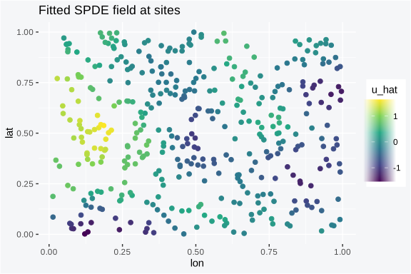

The fitted surface is a damped, smoothed version of the truth map from the simulation section: the SPDE prior pulls neighbouring sites together, so the recovered ripple has lower amplitude and softer edges than the field that generated the data, while keeping the location of the peaks and troughs.

Prediction

The continuous field buys something an areal model on these points could not: occupancy at coordinates that were never surveyed. The field is defined everywhere on the mesh, so a new location inside the mesh extent has a field value, interpolated from the node values through the same FEM basis that built the fit. Build a regular grid of prediction coordinates over the unit square, project the fitted node field onto it with a fresh projection matrix from tulpaMesh::fem_matrices(), and add it to the fixed-effect predictor.

grid <- expand.grid(lon = seq(0.05, 0.95, length.out = 30),
                    lat = seq(0.05, 0.95, length.out = 30))
A_new <- tulpaMesh::fem_matrices(mesh, obs_coords = as.matrix(grid))$A
field_new <- as.numeric(A_new %*% u_hat)
str(field_new)
#>  num [1:900] -0.863 -1.036 -1.202 -1.327 -1.283 ...

The fixed-effect part of the prediction comes from predict() with a design matrix at the new locations. Setting occ_cov to its mean isolates the spatial surface: the prediction is occupancy at an average-covariate site, varying only through the field. predict() returns the posterior mean, SD, and quantiles of psi from the fixed-effect draws, so the SD column carries the fixed-effect uncertainty, and the field is added on the logit scale before the inverse-link.

X0 <- cbind(1, rep(mean(dat$occ_cov), nrow(grid)))
pred_fixed <- predict(fit_sp, X.0 = X0)
eta_grid <- qlogis(pred_fixed$mean) + field_new
psi_grid <- plogis(eta_grid)
grid$psi <- psi_grid
summary(grid$psi)
#>    Min. 1st Qu.  Median    Mean 3rd Qu.    Max. 
#>  0.1073  0.2369  0.3110  0.3312  0.4046  0.6910

Mapping the predicted occupancy over the grid gives the continuous surface, filled in between the surveyed points. This is the deliverable a continuous field exists for: a smooth occupancy map at every coordinate, not just at the sites that happened to be visited.

ggplot(grid, aes(lon, lat, fill = psi)) +
  geom_raster() +
  geom_point(data = dat, aes(lon, lat), inherit.aes = FALSE,
             size = 0.4, colour = "white", alpha = 0.5) +
  scale_fill_viridis_c() +
  labs(title = "Predicted occupancy (mean covariate)", fill = "psi") +
  theme(panel.background = element_rect(fill = "transparent"),
        plot.background  = element_rect(fill = "transparent"))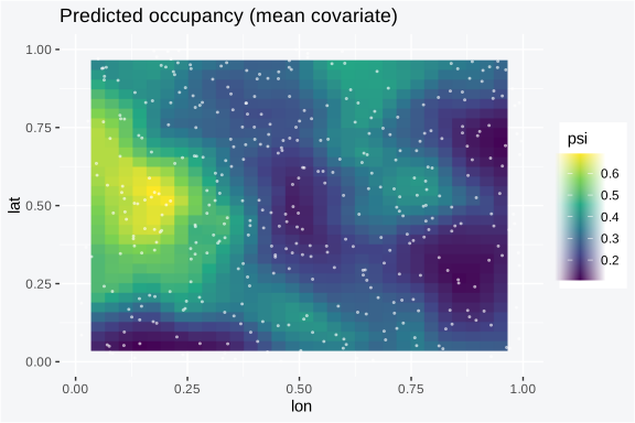

The fixed-effect SD in pred_fixed$sd propagates the coefficient uncertainty into the map, and a wider band appears where the data are sparse and the intercept is less pinned. The field’s own posterior uncertainty is not in this band: the Laplace path stores the field mode, not a per-node SD, so the interval here is conditional on the fitted field. For a fully marginalised field band on coordinates, the areal method = "nested_laplace" path computes a per-cell psi_lower / psi_upper directly; the continuous-field counterpart reports the mode.

Model comparison

In simulation a high correlation with a known truth says the field works. On real data there is no truth, so the question becomes whether the field improves prediction enough to justify the latent variables it adds. WAIC estimates out-of-sample predictive accuracy from the pointwise log-likelihood, lower is better, and it docks the model for the effective parameters it spends. One caveat applies here: the tulpaObs WAIC scores the fixed-effect predictor and does not fold the SPDE field contribution into the per-site likelihood, so on a spatial fit it is conditional on the fixed effects. It still answers whether the covariate-and-detection structure predicts the histories, and it is the apples-to-apples comparison against the non-spatial fit, which has no field either.

w_ns <- waic(fit_ns)
w_sp <- waic(fit_sp)
data.frame(
  model  = c("non_spatial", "spde"),
  waic   = round(c(w_ns$estimates["waic", "Estimate"], w_sp$estimates["waic", "Estimate"]), 1),
  p_waic = round(c(w_ns$estimates["p_waic", "Estimate"], w_sp$estimates["p_waic", "Estimate"]), 2),
  elpd   = round(c(w_ns$estimates["elpd_waic", "Estimate"], w_sp$estimates["elpd_waic", "Estimate"]), 1)
)
#>         model   waic p_waic   elpd
#> 1 non_spatial 1951.5   4.04 -975.7
#> 2        spde 1880.7   3.67 -940.4

The cleaner test for the field on these data is the residual diagnostic from the checking section: a non-spatial fit leaves spatial autocorrelation in its occupancy residuals, the SPDE fit removes it. That is the direct evidence the field is doing work, where WAIC on the fixed-effect predictor is the conditional view. Pairing the two, residual Moran’s I for whether the field is needed and WAIC for whether the mean structure predicts, is the honest read.

The comparison is asymmetric by design. WAIC and the residual test do not reward the field for flexibility alone; they reward it only for flexibility the data use. Had the simulated occupancy been spatially flat, the field would have found nothing to fit, the residual Moran’s I would have been non-significant in both fits, and the WAIC gap would have closed or reversed as the field’s extra latent variables bought no predictive gain. A model selection that punishes an unused field as readily as it credits a used one is the kind that keeps you honest on real data, where the truth map is unavailable and the only evidence is out-of-sample fit and leftover structure.

A second comparison is the field correlation itself, which only a simulation affords. The SPDE recovers the smooth surface at a correlation of roughly 0.4 to 0.5 with the truth at this sample size and mesh, where the non-spatial model has no surface to recover. Put the two evidence lines in one table.

data.frame(
  metric      = c("field cor (vs truth)", "WAIC (fixed-effect)"),
  non_spatial = c(NA_real_,    round(w_ns$estimates["waic", "Estimate"], 1)),
  spde        = c(round(corr, 3), round(w_sp$estimates["waic", "Estimate"], 1))
)
#>                 metric non_spatial     spde
#> 1 field cor (vs truth)          NA    0.652
#> 2  WAIC (fixed-effect)      1951.5 1880.700

The field correlation is the simulation-only number, available only for the SPDE fit since the non-spatial model has no surface to recover, and the WAIC is conditional on the fixed effects. Read alongside the residual Moran’s I from the check_model() output above, they say the field captured a real spatial signal that the non-spatial model could not, which is exactly how the data were built.

Practical guidance

A few rules of thumb for continuous occupancy fields, with the numbers that make them usable.

• Set the range prior to roughly a third of the study extent, then check. prior.range = c(0.3, 0.5) on a unit square says the median range is 0.3 of the domain, the distance over which sites stay correlated, with even odds it is smaller. A range much shorter than the typical inter-site spacing leaves the field unable to borrow strength (every site is effectively isolated); a range near the full extent makes the field nearly flat and indistinguishable from the intercept. Start at a third of the extent, fit, and look at the recovered field SD: if it collapses toward zero the prior range is fighting the data.

• Tie max.edge to the range, inner edge well below it. The mesh resolution has to be fine enough to represent the field’s wiggles. A useful default is an inner max.edge of one-fifth to one-third of the prior range, with the outer edge two to three times the inner so the buffer stays cheap. Here max.edge = c(0.3, 0.6) against a range of 0.3 is at the coarse end and gives a few hundred nodes; halving the inner edge to 0.15 roughly doubles the node count and sharpens the field, at a proportional cost in fit time. The N = 1500 recovery tier in the package’s own tests uses c(0.18, 0.45) for this reason.

• At least a few hundred sites, and detection that is not too sparse. The field’s range and marginal SD are learned from how occupancy varies across space, and a few dozen scattered points leave both barely informed. Below roughly 200 sites a continuous field is mostly prior, and a covariate-only fit is the more honest choice. The recovery here uses 400 sites with 8 visits at moderate detection; with very few visits or very low detection the model struggles to tell an unoccupied site from an occupied-but-undetected one, and the field inherits that ambiguity.

The decision between a continuous field and an areal field follows the data geometry:

Your sites	Field to use	Term	Engine
Raw coordinates on a continuous landscape	Matern SPDE	spde(lon, lat)	method = "laplace"
Regions joined by borders, graph given	ICAR / BYM2	icar(graph) / bym2(graph)	method = "nested_laplace"
Regions, autocorrelation strength of interest	proper CAR	car_proper(graph)	method = "nested_laplace"
No spatial signal in residuals	none	covariates only	method = "laplace"

On priors, the PC prior on (range, sigma) is weakly informative and the default usually suffices, but the range is the sensitive one. Refitting with the median range halved and doubled is the cheap sensitivity check: if the recovered field and the occupancy slope move little, the prior is not driving the answer; if the field SD swings with the prior range, the data are not informing the range and you should report that the field is prior-dominated. The fixed-effect prior is separate and threads through priors = occu_priors() if you want to tighten the detection intercept or break the psi-p identifiability ridge at small J; priors = FALSE recovers the unpenalised MAP.

Three cases call for a different tool. When a non-spatial fit leaves no spatial autocorrelation in its residuals (Moran’s I p-value above 0.05), the field adds latent variables for nothing and the WAIC will not improve; do not fit it. When the sites are genuinely areal, regions with shared borders rather than points, the adjacency graph carries information the SPDE throws away by treating centroids as bare coordinates, so use icar() or bym2() on the nested_laplace path instead. And when you need a fully marginalised credible band on the field at new coordinates rather than a point surface, the continuous Laplace path stores the field mode only; the areal nested path is the one that returns calibrated per-cell intervals today, so route through it if the field’s own uncertainty is the deliverable.

Two limitations of the current SPDE-Laplace path are worth stating plainly. The prior at the prior modes of (range, sigma) is what the engine uses; nested integration over those hyperparameters, which would propagate their uncertainty into the field band, lands in a later release. And detection-side SPDE is not plumbed for the Laplace engine, so keep the spde() term in the occupancy formula, not in detection.

References

• Lindgren, F., Rue, H., & Lindstrom, J. (2011). An explicit link between Gaussian fields and Gaussian Markov random fields: the stochastic partial differential equation approach. Journal of the Royal Statistical Society B, 73, 423-498.

• Simpson, D., Rue, H., Riebler, A., Martins, T. G., & Sorbye, S. H. (2017). Penalising model component complexity: a principled, practical approach to constructing priors. Statistical Science, 32, 1-28.

• ?tobs for the unified fitter and the in-formula spde() term.

• vignette("spatial-occupancy", package = "tulpaObs") for the areal ICAR / BYM2 / CAR fields on a neighbour graph.

• vignette("occupancy-vs-inla", package = "tulpaObs") for the non-spatial occupancy story.

• vignette("diagnostics", package = "tulpaObs") for posterior-predictive checks and spatial residual diagnostics.