Cover hurdle: tulpaObs vs INLA on simulated cover data • tulpaObs

tulpaObs::cover(response = "lognormal") fits a two-arm hurdle model: a binomial GLM on the occurrence indicator $\mathbf{1}\{y_i > 0\}$ , and a Gaussian GLM on $\log y_i$ over the positive subset, with the lognormal back-transform $E[y_i \mid y_i > 0] = \exp(\eta_i^{\text{pos}} + \sigma^2 / 2)$ applied at prediction time. The same generative model can be fit in INLA::inla() as two independent calls (Michael Glaser’s separate-hurdle workflow in example/MOT_abund_data.Rmd §“INLA hurdles”). This vignette compares the two on simulated data where the truth is known.

Michael’s joint model couples the two arms through one shared spatial field with INLA’s copy= mechanism (the cover arm’s field is a fitted scalar multiple of the occurrence arm’s). tulpaObs reproduces that coupling in two places. The closest analogue is the spatial cover() path: a bym2() / icar() / car() term on the latent-presence formula under method = "nested_laplace", which fits one shared areal field and a copy coefficient alpha across the occurrence and cover arms. occu_cover() is the further generalization that adds a replicated detection arm on top of that coupling. This vignette starts on the separate-fit case, where the two engines should agree closely, then walks the function mapping, two side-by-side fits, the algorithmic differences, and the cases where INLA remains the better tool.

Installation

install.packages("pak")
pak::pak("gcol33/tulpaObs")            # latest from GitHub
pak::pak("gcol33/tulpaObs@v0.1.1")     # a specific tagged release

Tagged releases are listed at https://github.com/gcol33/tulpaObs/releases.

pak resolves the dependency tree, pulling tulpa and tulpaMesh from the r-universe repository DESCRIPTION declares in Additional_repositories, at or above the Imports floor. A C++17 toolchain is needed (Rtools on Windows, Xcode CLI tools on macOS, r-base-dev on Linux); both tulpa and tulpaObs compile their backends on first install.

Function mapping

The table below maps the INLA constructs in Michael’s two workflows to their tulpaObs counterparts. The left block is the independent-arm path (two inla() calls vs one cover() call); the right block is the joint copy= path (one inla() list-model vs the spatial cover() / detection occu_cover() engine).

INLA construct	tulpaObs equivalent	Notes
`inla(occur ~ x, family = "binomial")`	`tobs(~ x, family = cover("lognormal"), y = cover)` (occurrence arm)	One `cover()` call fits both arms; no separate occurrence call.
`inla(log_cover ~ x, family = "gaussian", data = subset(occur == 1))`	the positive arm of the same `cover()` fit	tulpaObs subsets to `y > 0` internally inside `encode_cover_hurdle()`.
`family = "gaussian"` precision hyperparameter	`fit$sigma_pos` (residual SD, `1 / sqrt(precision)`)	tulpaObs reports the SD directly; INLA reports a precision posterior.
`family = c("binomial", "beta")` for cover in $(0, 1)$	`cover("beta")`	Logit-link beta with precision `phi`; see `fit$phi_pos`.
`f(site, model = "bym2", graph = adj)`	`bym2(graph = adj, group.var = "site")` in the formula	Areal field on the latent-presence linear predictor.
`f(site, model = "iid")`, `"besag"`, `"besagproper2"`	`icar(graph = adj)`, `car(graph = adj)`, `car_proper(graph = adj)`	One areal term per latent-presence formula.
`copy = "site", fixed = FALSE` (shared field, fitted scale)	the joint `cover()` path: `method = "nested_laplace"` with a `bym2()` term, copy coefficient `alpha`	`alpha` is integrated on the outer grid, surfaced as `fit$joint$theta_mean["alpha"]`.
`inla.stack()` for the joint design	not needed	tulpaObs builds the two-arm design from one formula and one `y`.
`control.compute = list(waic = TRUE)`	`waic(fit)`	WAIC on the assembled pointwise log-likelihood.
`inla.posterior.sample()` + manual differencing	`predict(fit, newdata, type = "expected")`	Posterior draws are differenced per draw inside `predict()`.
`pc.prec` / `pc` hyperpriors via `hyper = list(...)`	`cover_priors()` (fixed effects); `control$prior.sigma`, `control$prior.alpha` (joint hyperparameters)	Fixed-effect priors on both arms; PC-style amplitude / copy priors on the joint grid.
replicated detection: `inla()` has no native single-species detection arm	`occu_cover()` with a `detection` formula and an `N x J` visit matrix	The generalization INLA cannot express directly (see `example/info.md`).

Simulate

library(tulpaObs)

sim <- simulate_cover(
  N         = 400,
  beta.occ  = c(-0.4, 0.8),
  beta.pos  = c(-1.0, 0.3),
  sigma.pos = 0.4,
  seed      = 11
)

dat <- sim$data
dat$occur     <- as.integer(dat$cover > 0)
dat$log_cover <- ifelse(dat$cover > 0, log(dat$cover), NA_real_)

truth <- sim$truth
c(sum(dat$occur), mean(dat$occur))
#> [1] 165.0000   0.4125

The simulator’s truth$beta_occ, truth$beta_pos, and truth$sigma_pos give the parameters used to generate cover. Site-level prevalence mean(occur) lands near mean(plogis(eta_occ)) once enough sites are drawn. The generative model is exactly the one both engines target: a Bernoulli occurrence layer with a logit link, and a Gaussian layer on log(cover) for the occupied sites. Because the two layers are simulated independently here (no shared field), the separate-fit and the two-inla()-call workflows are fitting the same likelihood, and any gap in the recovery table is approximation error rather than model misspecification.

Fit with tulpaObs

fit_tulpa <- tobs(
  formula = ~ x,
  data    = dat,
  family  = cover(response = "lognormal"),
  y       = dat$cover
)
fit_tulpa
#> <cover_fit (lognormal positive part)>
#>   N total      : 400
#>   N positive   : 165 (41.2%)
#>   sigma_pos    : 0.4127
#>   converged    : yes
#> 
#> Presence (binomial logit):
#>               estimate   std.err   z.value
#> (Intercept) -0.3796073 0.1075194 -3.530594
#> x            0.7321596 0.1218140  6.010469
#> 
#> Positive (Gaussian on log y > 0):
#>               estimate    std.err    z.value
#> (Intercept) -1.0145209 0.03420426 -29.660658
#> x            0.3086659 0.03375217   9.145068

Fit with INLA (Michael’s separate-hurdle workflow)

library(INLA)
#> Loading required package: Matrix
#> This is INLA_25.10.19 built 2025-10-19 19:10:20 UTC.
#>  - See www.r-inla.org/contact-us for how to get help.
#>  - List available models/likelihoods/etc with inla.list.models()
#>  - Use inla.doc(<NAME>) to access documentation
#>  - Consider upgrading R-INLA to testing[26.08.22] or stable[26.08.07].

m_occ_inla <- INLA::inla(
  occur ~ x,
  family = "binomial",
  data   = dat,
  control.compute = list(waic = TRUE)
)

m_pos_inla <- INLA::inla(
  log_cover ~ x,
  family = "gaussian",
  data   = subset(dat, occur == 1),
  control.compute = list(waic = TRUE)
)

inla_beta_occ <- m_occ_inla$summary.fixed[, "mean"]
inla_beta_pos <- m_pos_inla$summary.fixed[, "mean"]

# Gaussian-arm residual SD from INLA's hyperpar (1 / sqrt(precision)).
inla_sigma_pos <- 1 / sqrt(
  m_pos_inla$summary.hyperpar["Precision for the Gaussian observations", "mean"]
)

Parameter recovery

recovery <- data.frame(
  parameter = c("beta_occ_0", "beta_occ_x",
                "beta_pos_0", "beta_pos_x",
                "sigma_pos"),
  truth     = c(truth$beta_occ, truth$beta_pos, truth$sigma_pos),
  tulpaObs  = c(fit_tulpa$beta_occ, fit_tulpa$beta_pos, fit_tulpa$sigma_pos),
  INLA      = c(inla_beta_occ,    inla_beta_pos,    inla_sigma_pos)
)
recovery$delta_tulpa <- recovery$tulpaObs - recovery$truth
recovery$delta_inla  <- recovery$INLA     - recovery$truth
recovery
#>    parameter truth   tulpaObs       INLA  delta_tulpa   delta_inla
#> 1 beta_occ_0  -0.4 -0.3796073 -0.3816751  0.020392720  0.018324926
#> 2 beta_occ_x   0.8  0.7321596  0.7393164 -0.067840445 -0.060683625
#> 3 beta_pos_0  -1.0 -1.0145209 -1.0145214 -0.014520890 -0.014521384
#> 4 beta_pos_x   0.3  0.3086659  0.3086657  0.008665909  0.008665746
#> 5  sigma_pos   0.4  0.4127451  0.4102460  0.012745070  0.010246036

Both engines hit the same fixed-effects estimates to within the Laplace/MAP vs. INLA-integrated marginal-mean tolerance. The two discrepancies that matter:

sigma_pos — tulpaObs computes the Gaussian residual SD post-hoc as sqrt(SS_res / (n - p)) because tulpa::tulpa_laplace(family = "gaussian") treats phi = 1 internally. INLA estimates the precision as a hyperparameter and reports its posterior mean. The two converge as n_positive grows.
beta_pos_0 — sensitive to the same Gaussian-precision detail; the intercept absorbs whatever residual scale the engine attributes to the data.

Predictive equivalence

newdata <- data.frame(x = seq(-2, 2, length.out = 50))

pred_tulpa <- data.frame(
  x       = newdata$x,
  E_cover = predict(fit_tulpa, newdata, type = "expected")
)

# INLA reconstruction: p * exp(eta_pos + sigma^2 / 2).
X <- model.matrix(~ x, newdata)
eta_occ_inla <- as.numeric(X %*% inla_beta_occ)
eta_pos_inla <- as.numeric(X %*% inla_beta_pos)
p_inla       <- plogis(eta_occ_inla)
mu_inla      <- exp(eta_pos_inla + inla_sigma_pos^2 / 2)
pred_inla    <- data.frame(x = newdata$x, E_cover = p_inla * mu_inla)

cor(pred_tulpa$E_cover, pred_inla$E_cover)
#> [1] 0.9999998
max(abs(pred_tulpa$E_cover - pred_inla$E_cover))
#> [1] 0.001122747

Both engines reconstruct expected cover the same way, E[y] = p * mu with mu = exp(eta_pos + sigma^2 / 2), so the curves track each other across the covariate range. The correlation is effectively one, and the maximum absolute gap traces back to the sigma_pos difference noted above: a small shift in the residual SD feeds through the lognormal back-transform and scales mu. On 400 sites with prevalence near 0.5 the gap stays a few percent of the predicted mean; it shrinks as the positive subset grows.

plot(pred_tulpa$x, pred_tulpa$E_cover, type = "l", lwd = 2,
     xlab = "x", ylab = "E[cover]",
     main = "Expected cover: tulpaObs (black) vs INLA (red)")
lines(pred_inla$x, pred_inla$E_cover, col = 2, lwd = 2, lty = 2)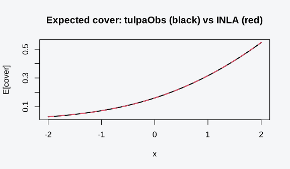

The joint copy= model side by side

The separate fits above ignore any shared structure between the two arms. Michael’s mod.joint model assumes the occurrence and cover signals respond to the same latent spatial field, and ties them with copy=. The tulpaObs analogue is the spatial cover() path: add a bym2() term to the formula and switch to method = "nested_laplace". The engine identifies one field z per region and writes eta_occ = X beta_occ + sigma * z, eta_pos = X beta_pos + alpha * sigma * z, integrating the copy coefficient alpha on the outer hyperparameter grid.

n_s <- 25L
adj <- matrix(0L, n_s, n_s)
for (s in seq_len(n_s)) {
  if (s > 1L)   adj[s, s - 1L] <- 1L
  if (s < n_s)  adj[s, s + 1L] <- 1L
}

sim_joint <- simulate_cover_joint(
  N        = 300L,
  adj      = adj,
  beta.occ = c(-0.3, 0.7),
  beta.pos = c(-1.5, -0.5),
  sigma    = 0.6,
  rho      = 0.7,
  alpha    = 1.0,
  positive = "lognormal",
  seed     = 21L
)

The simulate_cover_joint() generator demeans both BYM2 sub-blocks before scaling, matching the sum-to-zero constraint the engine applies, so the recovered cover-arm intercept targets the population truth rather than a field-mean offset. The cover-arm intercept sits well below zero so the lognormal median stays under the cover ceiling of 1: the generator caps its draws there, and an intercept near or above the ceiling censors most of the positive responses and flattens the cover-arm slope. The truth carries sigma = 0.6, alpha = 1.0 (the two arms see the field identically), and sigma_pos = alpha * sigma. The same demeaning matters in INLA: a bym2 field there is also sum-to-zero constrained, so a simulator that skips the demean biases the intercept in INLA the same way it does here. The constrained field causes it; the behaviour is identical across both implementations.

fit_joint <- tobs(
  formula = ~ x + bym2(graph = adj, group.var = "region") +
              share(spatial(), alpha = grid(c(0.25, 0.75, 1.5, 2.5))),
  data    = sim_joint$data,
  family  = cover("lognormal"),
  y       = sim_joint$y,
  method  = "nested_laplace",
  control = list(
    sigma.grid = c(0.4, 0.8),
    rho.grid   = c(0.5, 0.9),
    verbose    = FALSE
  )
)
#> [nested-laplace-joint] 1/112 cells (1%) | elapsed 0s | ETA >=0s | 0.00s/cells
#> [nested-laplace-joint] 11/11 cells (100%) | elapsed 0s | ETA done | 0.00s/cells
#> [nested-laplace-joint] 1/18 cells (6%) | elapsed 0s | ETA >=0s | 0.00s/cells
#> [nested-laplace-joint] 5/5 cells (100%) | elapsed 0s | ETA done | 0.00s/cells
#> [nested-laplace-joint] 1/3 cells (33%) | elapsed 0s | ETA >=0s | 0.00s/cells
#> [nested-laplace-joint] 1/1 cells (100%) | elapsed 0s | ETA done | 0.00s/cells
#> [nested-laplace-joint] 1/16 cells (6%) | elapsed 0s | ETA >=0s | 0.00s/cells
#> [nested-laplace-joint] 8/8 cells (100%) | elapsed 0s | ETA done | 0.00s/cells
#> [nested-laplace-joint] 1/12 cells (8%) | elapsed 0s | ETA >=0s | 0.00s/cells
#> [nested-laplace-joint] 1/1 cells (100%) | elapsed 0s | ETA done | 0.00s/cells
#> [nested-laplace-joint] 1/15 cells (7%) | elapsed 0s | ETA >=0s | 0.00s/cells
#> [nested-laplace-joint] 8/8 cells (100%) | elapsed 0s | ETA done | 0.00s/cells
#> [nested-laplace-joint] 1/4 cells (25%) | elapsed 0s | ETA >=0s | 0.00s/cells
#> [nested-laplace-joint] 1/1 cells (100%) | elapsed 0s | ETA done | 0.00s/cells
#> [nested-laplace-joint] 1/20 cells (5%) | elapsed 0s | ETA >=0s | 0.00s/cells
#> [nested-laplace-joint] 12/12 cells (100%) | elapsed 0s | ETA done | 0.00s/cells
#> [nested-laplace-joint] 1/18 cells (6%) | elapsed 0s | ETA >=0s | 0.00s/cells
#> [nested-laplace-joint] 1/1 cells (100%) | elapsed 0s | ETA done | 0.01s/cells
#> [nested-laplace-joint] 1/32 cells (3%) | elapsed 0s | ETA >=0s | 0.00s/cells
#> [nested-laplace-joint] 21/21 cells (100%) | elapsed 0s | ETA done | 0.00s/cells
#> [nested-laplace-joint] 1/16 cells (6%) | elapsed 0s | ETA >=0s | 0.00s/cells
#> [nested-laplace-joint] 1/1 cells (100%) | elapsed 0s | ETA done | 0.00s/cells
#> [nested-laplace-joint] 1/32 cells (3%) | elapsed 0s | ETA >=0s | 0.00s/cells
#> [nested-laplace-joint] 20/20 cells (100%) | elapsed 0s | ETA done | 0.00s/cells
#> [nested-laplace-joint] 1/10 cells (10%) | elapsed 0s | ETA >=0s | 0.00s/cells
#> [nested-laplace-joint] 1/1 cells (100%) | elapsed 0s | ETA done | 0.00s/cells

joint_recovery <- data.frame(
  parameter = c("beta_occ_x", "beta_pos_x", "alpha", "sigma"),
  truth     = c(sim_joint$truth$beta_occ[2], sim_joint$truth$beta_pos[2],
                sim_joint$truth$alpha,       sim_joint$truth$sigma),
  estimate  = c(fit_joint$beta_occ[2], fit_joint$beta_pos[2],
                unname(fit_joint$joint$theta_mean["alpha"]),
                unname(fit_joint$joint$theta_mean["sigma"]))
)
joint_recovery
#>    parameter truth   estimate
#> 1 beta_occ_x   0.7  0.6579782
#> 2 beta_pos_x  -0.5 -0.4723106
#> 3      alpha   1.0  1.1124143
#> 4      sigma   0.6  0.7026160

The occurrence and cover slopes land on the right side of zero (truth +0.7 and -0.5), and alpha recovers near its true 1.0. The estimate of sigma reads off the field amplitude on the occurrence arm; the cover arm sees the same field at alpha * sigma. With only 25 regions the field-level quantities (alpha, sigma) carry visible sampling noise; the fixed-effect slopes, which pool over all 300 sites, recover more tightly. This is the same small-region behaviour Michael’s MOTIVATE fit shows, and it is intrinsic to the data, not to the engine.

The same model in INLA is a single inla() call over an inla.stack() that lays the binomial and Gaussian responses on a shared index, with the cover arm’s field declared as a copy of the occurrence arm’s. The copy weight is the fitted scalar Beta for ... hyperparameter, the direct counterpart of tulpaObs’s alpha.

# Joint shared-field hurdle in INLA (Michael's mod.joint pattern). Not run
# here (INLA may be absent at build); shown for the structural mapping.
#
# n <- nrow(sim_joint$data)
# occur     <- as.integer(sim_joint$y > 0)
# log_cover <- ifelse(sim_joint$y > 0, log(sim_joint$y), NA_real_)
# site      <- as.integer(sim_joint$data$region)
#
# # Two-column response: occurrence in col 1, log-cover in col 2.
# Y <- matrix(NA_real_, 2 * n, 2)
# Y[1:n,        1] <- occur
# Y[(n + 1):(2 * n), 2] <- log_cover
#
# stk <- inla.stack(
#   data = list(Y = Y),
#   A    = list(1),
#   effects = list(list(
#     occ_int = c(rep(1, n), rep(NA, n)),
#     pos_int = c(rep(NA, n), rep(1, n)),
#     x_occ   = c(sim_joint$data$x, rep(NA, n)),
#     x_pos   = c(rep(NA, n), sim_joint$data$x),
#     s_occ   = c(site, rep(NA, n)),
#     s_pos   = c(rep(NA, n), site)
#   ))
# )
#
# joint <- inla(
#   Y ~ -1 + occ_int + pos_int + x_occ + x_pos +
#       f(s_occ, model = "bym2", graph = adj) +
#       f(s_pos, copy = "s_occ", fixed = FALSE),
#   family = c("binomial", "gaussian"),
#   data   = inla.stack.data(stk),
#   control.predictor = list(A = inla.stack.A(stk))
# )
# joint$summary.hyperpar["Beta for s_pos", "mean"]   # the copy coefficient

The structural difference is visible in the two code blocks. tulpaObs reads one formula and one response vector; the two-arm design, the subset-to-positive, and the shared-field bookkeeping happen inside the dispatcher. INLA needs the response stacked into a two-column matrix, each fixed effect split into an occurrence column and a cover column, and the field declared once and copied. The occu_cover() family extends the tulpaObs side one step further: it adds an N x J detection matrix and a detection formula so each cell’s presence is observed through replicated visits, a structure the copy= stack does not express because INLA has no native single-species detection arm.

Key differences

Algorithm. INLA runs nested Laplace approximation throughout: a Laplace approximation to the latent field conditional on hyperparameters, then a grid or CCD integration over the hyperparameters, with no exact-MCMC step. The separate cover() path runs two independent Laplace approximations through tulpa::tulpa_laplace() (binomial on occurrence, Gaussian on log-cover); the joint cover() path runs tulpa::tulpa_nested_laplace_joint(), which is the same nested-Laplace recipe INLA uses, integrating (sigma, alpha, phi) on an outer grid with an inner Newton solve per cell. The two engines therefore agree closely on the means for these Gaussian-latent blocks, which is what the recovery table shows.

Speed. For the separate-fit case both engines finish in well under a second on 400 sites; the cost is dominated by the design-matrix algebra, not the optimizer. For the joint shared-field case the cost is the outer grid size: the example above pins a small one, which keeps the fit fast, but a dense default grid with adaptive densification runs longer. tulpaObs exposes the grid directly through control$sigma.grid, control$rho.grid, and the share() amplitude, so the time-accuracy trade is in the user’s hands.

Output format. INLA returns full posterior marginals for every fixed effect and hyperparameter (summary.fixed, summary.hyperpar, plus the marginal densities). tulpaObs returns a cover_fit object carrying beta_occ / beta_pos with Hessian-based or grid-integrated SEs, the dispersion summary (sigma_pos or phi_pos), and posterior draws reachable through predict(). The joint fit additionally exposes the outer-grid hyperparameter posterior under fit$joint$theta_mean and fit$joint$theta_grid, where alpha and sigma_occ live. The grid is the explicit object INLA hides behind its CCD integrator: each row of theta_grid is one hyperparameter cell, and fit$joint$weights gives its posterior mass. Reading theta_mean is a weighted average over those cells, so a flat grid signals an under-resolved posterior the same way a concentrated one signals a well-identified hyperparameter. When the team’s question is the copy coefficient itself (does the cover signal track the occurrence signal, and by how much), alpha and its grid are the answer the joint fit was built to give.

Prior specification. INLA places PC priors on the hyperparameters through the hyper = list(...) argument of each f() term and Gaussian priors on fixed effects through control.fixed. tulpaObs splits the same two concerns: cover_priors() carries the fixed-effect Gaussian penalty for both arms, and the joint hyperparameters take PC-style priors through control$prior.sigma (field amplitude) and control$prior.alpha (the copy coefficient). The alpha prior is the direct regularizer on the copy scalar at small n_positive, the role INLA’s copy hyperprior plays.

Shared-field coupling. This is the substantive modelling difference. INLA’s copy= declares the cover arm’s field to be a scalar multiple of the occurrence arm’s: the field pattern is locked across arms and only the magnitude Beta for ... is fitted. The tulpaObs joint cover() path encodes the identical structure with alpha, eta_pos = X beta_pos + alpha * sigma * z, and integrates alpha over the outer grid rather than optimizing a single hyperparameter mode. The separate-fit cover() path used in the recovery table does not couple the arms at all, which is why it is the right baseline for the agreement check and the wrong tool when the shared-field signal is real. occu_cover() keeps the same alpha coupling and adds the detection arm on top.

When NOT to switch

INLA is the better tool in several honest cases, and the migration is not worth the effort when one of these holds.

You need full posterior marginals, not summaries. INLA hands back the marginal density of every fixed effect and hyperparameter, ready for inla.tmarginal() transforms, tail-probability queries, and exact credible intervals on derived quantities. tulpaObs returns posterior draws and moment summaries; if your downstream work differences or transforms marginals heavily and you want INLA’s smoothed densities rather than draws, staying in INLA avoids re-deriving that layer.

Your latent structure is one INLA already ships and tulpaObs does not. INLA’s f() library covers SPDE continuous-space fields, rw1 / rw2 smoothers, ar1, seasonal, rgeneric user blocks, and a large catalogue of built-in models. The tulpaObs cover engine couples areal bym2() / icar() / car() / car_proper() fields and the Mundlak within-between temporal decomposition. If your model needs a structure outside that set, INLA expresses it today and the tulpaObs port would be new engine code.

You are coupling more than two arms, or arms tulpaObs does not model. The copy= mechanism generalizes to many linear predictors sharing many fields with independent copy weights. The tulpaObs joint engine couples the occurrence and cover arms (and, in occu_cover(), the detection arm) through the shared field; a three-or-more-likelihood integrated model with several copied fields is INLA territory.

Your team’s pipeline is already INLA. Michael’s MOTIVATE workflow runs inla.stack(), inla.posterior.sample(), and the copy= joint fit end to end. If the goal is to reproduce or extend that exact pipeline rather than start fresh, the cost of rebuilding the stack-and-sample plumbing in tulpaObs usually outweighs the gain. The migration pays off when you want the replicated detection arm, exact-MCMC debiasing of the Laplace body, or the single-formula interface, none of which the copy= stack provides.

When the two diverge

The two engines diverge in three places that the separate-fit story doesn’t surface:

Joint shared spatial field. Michael’s mod.joint/copy= model forces the cover linear predictor’s spatial component to be a scalar multiple of the occurrence linear predictor’s – pattern locked, magnitude fitted. The separate-fit cover() path compared in the recovery table does not couple the two arms; the spatial cover() joint path shown above (a fitted copy coefficient alpha on a shared field) is the coupled analogue, and occu_cover() adds a detection arm on top.
Beta positive part. Michael’s joint model uses family = c("binomial", "beta") for cover in $(0, 1)$ on the natural scale; cover("beta") and occu_cover("beta") are the tulpaObs equivalents.
Uncertainty propagation. INLA returns full posterior marginals on both arms; the separate-fit path here returns the Laplace mode and a Hessian-based SE per arm. The two agree on the means within sampling noise but diverge on tail behaviour for small n_positive.

References

example/MOT_abund_data.Rmd §“INLA hurdles” — Michael Glaser’s separate-hurdle and joint-copy= workflows on the MOTIVATE resurvey data.
example/info.md — Michael’s note on why a proper single-species occupancy model is hard in INLA (the marginalization problem).
vignette("cover-hurdle-motivate") — the joint shared-field cover model and the beta positive variant on a resurvey panel.
vignette("cover-hurdle") — the independent-arm dispatcher in isolation.