Cover hurdle on resurvey panels (MOTIVATE reduction)

Installation

install.packages("pak")
pak::pak("gcol33/tulpaObs")            # latest from GitHub
pak::pak("gcol33/tulpaObs@v0.1.1")     # a specific tagged release

Tagged releases are listed at https://github.com/gcol33/tulpaObs/releases.

pak resolves the dependency tree, pulling tulpa and tulpaMesh from the r-universe repository DESCRIPTION declares in Additional_repositories, at or above the Imports floor. A C++17 toolchain is needed (Rtools on Windows, Xcode CLI tools on macOS, r-base-dev on Linux); both tulpa and tulpaObs compile their backends on first install.

Introduction

Vegetation cover is a zero-inflated quantity. A plot either holds a species or it does not, and where the species is present, its cover lands somewhere in $(0, 1]$ . Two questions ride on the same data: where does the species occur, and how much of it is there once it occurs. A naive Gaussian or beta regression on cover mixes the two, because the zeros and the positive values answer different questions. A hurdle model separates them into an occurrence arm and a positive-cover arm.

The two arms are not independent. A patch of habitat that lifts the chance of presence usually also lifts the cover where the species is present: the same soil moisture, the same grazing history, the same nutrient gradient drives both. tulpaObs couples the arms through one shared spatial field. The occurrence arm sees the field at full amplitude; the cover arm sees a scalar multiple of it, with the multiplier (the copy coefficient) fitted from the data rather than assumed. Fitting the two arms separately throws this coupling away. It also wastes the cover observations: a plot with high cover is evidence that the latent field is high there, which sharpens the occurrence estimate at neighbouring plots, and the separate fit never propagates that. The joint fit borrows strength across arms and across space at once, and it reports the copy coefficient with a credible interval so you can ask whether the two processes really do track each other.

There is a third reason the joint model matters, specific to monitoring. When the goal is to estimate change, not just a snapshot, the coupling decides how a shift in occurrence translates into a shift in cover. If a warming climate lifts the occurrence probability at a plot, the joint model says cover there rises too, by an amount the copy coefficient sets; the separate model leaves the two changes unlinked and can report a rising occurrence beside a flat cover with no internal contradiction. Whether that linkage is real is an empirical question, and the joint fit answers it with the posterior on the copy coefficient rather than forcing it to zero (separate fits) or to one (hard-copied fits).

This vignette builds the joint cover-hurdle end to end on a reduced generator that mimics the structure of the MOTIVATE resurvey workflow: plots laid out in space (BYM2 adjacency), visited at irregular intervals across decades, with vegetation cover recorded on the natural $[0, 1]$ scale. It then switches to the three-arm occu_cover() family, which adds an explicit detection layer and the change-quantity prediction contract the resurvey literature wants. The two families share an engine and a parameterization; the difference is whether you trust your zeros. If a zero always means true absence, the two-arm cover() family is enough. If a zero can mean the species was there and missed, the three-arm occu_cover() family separates non-detection from absence and the detection arm earns its parameters.

The reduction stays in synthetic territory so the vignette is reproducible and CRAN-safe; the full MOTIVATE comparison runs as a local script under dev_notes/.

The model

Write $y_i$ for the cover at observation $i$ , on the natural $[0, 1]$ scale, with $y_i = 0$ recording absence. The hurdle splits into an occurrence indicator and a positive part. Let $z_i = \mathbf{1}\{y_i > 0\}$ be the occurrence indicator with probability $p_i$ , and let the positive cover follow a family $f$ (lognormal on $\log y_i$ , or beta on $y_i$ directly):

$z_i \sim \mathrm{Bernoulli}(p_i), \qquad \operatorname{logit} p_i = \mathbf{x}_i^\top \boldsymbol\beta^{\mathrm{occ}} + w_{s(i)},$ $y_i \mid z_i = 1 \sim f\!\left(\eta_i^{\mathrm{pos}}, \theta\right), \qquad \eta_i^{\mathrm{pos}} = \mathbf{x}_i^\top \boldsymbol\beta^{\mathrm{pos}} + \alpha\, w_{s(i)} .$

Here $w_s$ is a BYM2 field over the spatial units $s$ , with marginal amplitude $\sigma$ and ICAR/IID mixing $\rho$ , mapped to observation $i$ through $s(i)$ . The occurrence arm loads the field at amplitude one; the cover arm loads the same field scaled by $\alpha$ , the copy coefficient. So $\alpha = 1$ means the two arms see the field identically, $\alpha = 0$ decouples them (the cover arm has no shared spatial structure), and a negative $\alpha$ means the two processes run in opposition. The dispersion $\theta$ is the beta precision $\phi$ or the lognormal residual SD $\sigma_{\mathrm{pos}}$ , depending on the positive family. The symbol $w_{s(i)}$ is the single object that turns two regressions into a joint model: it is shared, and only its amplitude on the cover arm is free.

The copy coefficient is what makes this a joint model rather than two regressions stapled together. With $\alpha$ free, the cover observations inform the field, and the field informs occurrence: a plot with high cover pushes $w_s$ up there, which raises $\psi$ at that plot and, through the ICAR penalty, at its neighbours. Information flows both ways across the arms and across space. A separate fit severs the cross-arm path entirely, and a hard-copied fit ( $\alpha$ fixed at one) assumes the flow is at full strength without checking. The free copy coefficient sits between those two and lets the data set the strength.

The latent $z_i$ marginalises out of the likelihood in closed form (two states per observation), so the fit is a nested Laplace approximation, with the hyperparameters $(\sigma, \alpha, \theta)$ integrated on an outer grid and the field plus coefficients solved by an inner Newton step at each grid point. That is the joint engine, the default for method = "nested_laplace" on occu_cover(). Because the hyperparameters are integrated rather than optimized, the SEs on $\alpha$ and $\sigma$ reflect the full posterior over the grid, not a curvature approximation at a single mode, and the coefficient SEs fold in the uncertainty about the field amplitude through the law of total variance. The price is that the outer grid has to be wide enough to bracket the posterior mass; a grid that clips the mode biases the integrated estimate, a point the practical guidance returns to.

A MOTIVATE-style simulator

simulate_motivate <- function(n_plots        = 25L,
                              n_years        = 4L,
                              year_step      = 5,
                              baseline_range = c(0, 10),
                              intercept_occ  = -0.3,
                              intercept_pos  = -1.5,
                              beta_occ_btw   = -0.05,
                              beta_occ_wtn   =  0.10,
                              beta_pos_btw   = -0.02,
                              beta_pos_wtn   =  0.05,
                              alpha          = 1.0,
                              sigma          = 0.6,
                              rho            = 0.7,
                              phi            = 30,
                              sigma_pos_ln   = 0.4,
                              positive       = c("beta", "lognormal"),
                              seed           = NULL) {
  positive <- match.arg(positive)
  if (!is.null(seed)) set.seed(seed)

  adj <- matrix(0L, n_plots, n_plots)
  for (s in seq_len(n_plots)) {
    if (s > 1L)       adj[s, s - 1L] <- 1L
    if (s < n_plots)  adj[s, s + 1L] <- 1L
  }

  iid <- stats::rnorm(n_plots, 0, 1)
  spa <- stats::rnorm(n_plots, 0, 1)
  w_occ <- sigma * (sqrt(rho) * spa + sqrt(1 - rho) * iid)
  w_pos <- alpha * w_occ

  baselines <- stats::runif(n_plots, baseline_range[1], baseline_range[2])
  plot_rows <- lapply(seq_len(n_plots), function(p) {
    data.frame(
      plot_id = factor(p, levels = seq_len(n_plots)),
      year    = baselines[p] + (seq_len(n_years) - 1L) * year_step
    )
  })
  dat <- do.call(rbind, plot_rows)

  yr_btw <- stats::ave(dat$year, dat$plot_id, FUN = mean)
  yr_wtn <- dat$year - yr_btw
  yr_btw_c <- yr_btw - mean(c(baseline_range))

  idx <- as.integer(dat$plot_id)
  eta_occ <- intercept_occ +
    beta_occ_btw * yr_btw_c + beta_occ_wtn * yr_wtn + w_occ[idx]
  eta_pos <- intercept_pos +
    beta_pos_btw * yr_btw_c + beta_pos_wtn * yr_wtn + w_pos[idx]

  p_occ <- stats::plogis(eta_occ)
  occur <- stats::rbinom(nrow(dat), 1L, p_occ)
  y <- numeric(nrow(dat))
  is_pos <- occur == 1L
  if (positive == "beta") {
    mu_pos <- stats::plogis(eta_pos)
    y[is_pos] <- stats::rbeta(sum(is_pos),
                              mu_pos[is_pos] * phi,
                              (1 - mu_pos[is_pos]) * phi)
  } else {
    log_cov <- stats::rnorm(sum(is_pos), eta_pos[is_pos], sigma_pos_ln)
    y[is_pos] <- exp(log_cov)
  }
  y <- pmin(pmax(y, 0), 1 - 1e-6)

  list(
    data  = dat,
    y     = y,
    adj   = adj,
    truth = list(
      beta_occ_btw = beta_occ_btw, beta_occ_wtn = beta_occ_wtn,
      beta_pos_btw = beta_pos_btw, beta_pos_wtn = beta_pos_wtn,
      alpha = alpha, sigma = sigma, rho = rho,
      phi = phi, sigma_pos_ln = sigma_pos_ln,
      positive = positive,
      w_occ = w_occ, w_pos = w_pos,
      baselines = baselines
    )
  )
}

The simulator places plots on a chain adjacency (BYM2’s simplest geometry), draws a baseline year per plot uniformly over the resurvey window, and visits each plot at n_years evenly-spaced occasions starting from that baseline. The occurrence and positive-cover linear predictors share a BYM2 plot-level field scaled by alpha on the positive arm. The known truth is in sim$truth: occurrence slopes (beta_occ_btw, beta_occ_wtn), positive-cover slopes (beta_pos_btw, beta_pos_wtn), the copy coefficient alpha, the field amplitude sigma, the BYM2 mixing rho, and the per-plot field draws w_occ on the occurrence arm and w_pos = alpha * w_occ on the cover arm. Holding those fixed across two seeds lets us isolate the effect of the positive family: the beta and lognormal panels below share an identical occurrence layer and differ only in how the positive cover is drawn.

The field construction deserves a second look because it is the part most people get wrong. The occurrence-arm field w_occ is drawn once per plot as a BYM2-style mix of a spatially-structured component and an IID component, weighted by rho, and scaled by sigma. The cover-arm field is not redrawn: it is alpha * w_occ, the same field at a different amplitude. That is the copy structure made explicit in the generator. If you instead drew an independent field for the cover arm, you would be simulating the separate-fit world, and no joint model could recover an alpha, because there would be no shared field to scale. The two arms also carry their own within-plot and between-plot slopes, so the simulator can produce a species whose occurrence trends one way over time while its conditional cover trends another, which is the realistic case the Mundlak split is built to disentangle.

The two signals in `year`

A column called year in a resurvey table carries two distinct quantities:

Between-plot. Plots that were first surveyed in 1985 versus 2005 differ for reasons that have nothing to do with temporal change: selection criteria, study designs, or accessible regions shift over decades. Cross-plot baseline year is a site-property covariate.
Within-plot. A single plot’s cover at resurvey, controlling for that plot’s baseline, is the actual temporal trajectory.

A single slope on raw year mixes the two. The Mundlak decomposition (Mundlak 1978; Bell & Jones 2015) splits year into a per-plot mean (between) and the deviation from that mean (within), and the regression recovers a separate slope for each. tulpaObs::within_between() implements the split.

Generate two panels

library(tulpaObs)

sim_beta <- simulate_motivate(positive = "beta",      seed = 2026L)
sim_ln   <- simulate_motivate(positive = "lognormal", seed = 2026L)

c(n_rows        = nrow(sim_beta$data),
  n_plots       = nlevels(sim_beta$data$plot_id),
  prevalence_b  = mean(sim_beta$y > 0),
  prevalence_ln = mean(sim_ln$y   > 0))
#>        n_rows       n_plots  prevalence_b prevalence_ln 
#>        100.00         25.00          0.37          0.37

Each panel is 25 plots x 4 visits = 100 rows. The two simulations use the same seed so the occurrence layer is identical between them; only the positive-cover layer differs.

Within-between decomposition

dat_beta <- within_between(sim_beta$data, group = "plot_id", vars = "year")
dat_ln   <- within_between(sim_ln$data,   group = "plot_id", vars = "year")

head(dat_beta, 8)
#>   plot_id      year  year_btw year_wtn
#> 1       1  1.210209  8.710209     -7.5
#> 2       1  6.210209  8.710209     -2.5
#> 3       1 11.210209  8.710209      2.5
#> 4       1 16.210209  8.710209      7.5
#> 5       2  8.308465 15.808465     -7.5
#> 6       2 13.308465 15.808465     -2.5
#> 7       2 18.308465 15.808465      2.5
#> 8       2 23.308465 15.808465      7.5

year_btw is constant within each plot (the per-plot mean of visit years); year_wtn is the visit-level deviation from that mean. By construction year == year_btw + year_wtn, and year_wtn sums to zero within every plot.

Fitting the model

The BYM2 plot-level field is written into the formula as a bym2() term. The graph is over plots, so the term carries group.var = "plot_id" to map each visit row to its plot. The positive family is chosen by cover("beta") or cover("lognormal"), the cover values pass through y, and method = "nested_laplace" selects the joint shared-field engine. Everything else is a default: the field amplitude sigma, the copy coefficient alpha, the BYM2 mixing rho, and the dispersion are integrated on the outer hyperparameter grid.

fit_beta <- tobs(
  formula   = ~ year_btw + year_wtn +
               bym2(graph = sim_beta$adj, group.var = "plot_id"),
  data      = dat_beta,
  family    = cover("beta"),
  y         = sim_beta$y,
  method    = "nested_laplace",
  control   = list(verbose = FALSE)
)
#> [nested-laplace-joint] 1/210 cells (0%) | elapsed 0s | ETA >=0s | 0.00s/cells
#> [nested-laplace-joint] 24/24 cells (100%) | elapsed 0s | ETA done | 0.00s/cells
#> [nested-laplace-joint] 1/46 cells (2%) | elapsed 0s | ETA >=0s | 0.00s/cells
#> [nested-laplace-joint] 31/31 cells (100%) | elapsed 0s | ETA done | 0.00s/cells
#> [nested-laplace-joint] 1/60 cells (2%) | elapsed 0s | ETA >=0s | 0.00s/cells
#> [nested-laplace-joint] 46/46 cells (100%) | elapsed 0s | ETA done | 0.00s/cells
#> [nested-laplace-joint] 1/8 cells (13%) | elapsed 0s | ETA >=0s | 0.00s/cells
#> [nested-laplace-joint] 1/1 cells (100%) | elapsed 0s | ETA done | 0.00s/cells
#> [nested-laplace-joint] 1/120 cells (1%) | elapsed 0s | ETA >=0s | 0.00s/cells
#> [nested-laplace-joint] 98/98 cells (100%) | elapsed 0s | ETA done | 0.00s/cells
#> [nested-laplace-joint] 1/12 cells (8%) | elapsed 0s | ETA >=0s | 0.00s/cells
#> [nested-laplace-joint] 1/1 cells (100%) | elapsed 0s | ETA done | 0.00s/cells
fit_beta
#> <cover_fit (beta positive part)>
#>   N total      : 100
#>   N positive   : 37 (37.0%)
#>   phi_pos      : 12.5112
#>   converged    : yes
#> 
#> Presence (binomial logit):
#>                estimate    std.err    z.value
#> (Intercept) -0.97683827 1.02788099 -0.9503418
#> year_btw     0.03418019 0.08738402  0.3911492
#> year_wtn     0.11285528 0.04031103  2.7996131
#> 
#> Positive (beta, logit link, on y > 0):
#>                estimate    std.err    z.value
#> (Intercept) -0.96631233 0.48133867 -2.0075518
#> year_btw    -0.03366500 0.04076841 -0.8257619
#> year_wtn     0.05507153 0.02259020  2.4378506

The print method lays out both arms. The occurrence block is the binomial-logit fit on $z_i$ ; the cover block is the beta fit (logit link on the conditional mean) over the positive subset. The header carries the positive family, the total and positive sample sizes, the fitted dispersion (phi_pos for beta, sigma_pos for lognormal), and the convergence flag. The same call with the lognormal family fits the second panel:

fit_ln <- tobs(
  formula   = ~ year_btw + year_wtn +
               bym2(graph = sim_ln$adj, group.var = "plot_id"),
  data      = dat_ln,
  family    = cover("lognormal"),
  y         = sim_ln$y,
  method    = "nested_laplace",
  control   = list(verbose = FALSE)
)
#> [nested-laplace-joint] 1/210 cells (0%) | elapsed 0s | ETA >=0s | 0.00s/cells
#> [nested-laplace-joint] 32/32 cells (100%) | elapsed 0s | ETA done | 0.00s/cells
#> [nested-laplace-joint] 1/46 cells (2%) | elapsed 0s | ETA >=0s | 0.00s/cells
#> [nested-laplace-joint] 37/37 cells (100%) | elapsed 0s | ETA done | 0.00s/cells
#> [nested-laplace-joint] 1/8 cells (13%) | elapsed 0s | ETA >=0s | 0.00s/cells
#> [nested-laplace-joint] 1/1 cells (100%) | elapsed 0s | ETA done | 0.00s/cells
#> [nested-laplace-joint] 1/76 cells (1%) | elapsed 0s | ETA >=0s | 0.00s/cells
#> [nested-laplace-joint] 63/63 cells (100%) | elapsed 0s | ETA done | 0.00s/cells
#> [nested-laplace-joint] 1/8 cells (13%) | elapsed 0s | ETA >=0s | 0.00s/cells
#> [nested-laplace-joint] 1/1 cells (100%) | elapsed 0s | ETA done | 0.00s/cells
#> [nested-laplace-joint] 1/82 cells (1%) | elapsed 0s | ETA >=0s | 0.00s/cells
#> [nested-laplace-joint] 72/72 cells (100%) | elapsed 0s | ETA done | 0.00s/cells
#> [nested-laplace-joint] 1/14 cells (7%) | elapsed 0s | ETA >=0s | 0.00s/cells
#> [nested-laplace-joint] 1/1 cells (100%) | elapsed 0s | ETA done | 0.00s/cells
fit_ln
#> <cover_fit (lognormal positive part)>
#>   N total      : 100
#>   N positive   : 37 (37.0%)
#>   sigma_pos    : 0.6374
#>   converged    : yes
#> 
#> Presence (binomial logit):
#>                estimate    std.err   z.value
#> (Intercept) -0.97691500 1.02827530 -0.950052
#> year_btw     0.03418413 0.08741872  0.391039
#> year_wtn     0.11286076 0.04031254  2.799644
#> 
#> Positive (Gaussian on log y > 0):
#>                estimate    std.err    z.value
#> (Intercept) -1.27398815 0.47642097 -2.6740807
#> year_btw    -0.01455187 0.04039944 -0.3601997
#> year_wtn     0.05739005 0.02174242  2.6395432

Each fit exposes the coefficients and SEs per arm in beta_occ / se_occ and beta_pos / se_pos, the dispersion in sigma_pos / phi_pos (with the posterior SD in sigma_pos_sd / phi_pos_sd), and the raw joint engine result in fit$joint. The copy coefficient and donor amplitude come off the joint engine’s hyperparameter posterior, fit$joint$theta_mean, under the names alpha and sigma_occ.

Exact row reduction

The joint engine collapses each arm to its exact sufficient statistic before the inner solve. Plots that share the occurrence design row and every per-observation latent component (the spatial cell, the trend weight) are exchangeable Bernoulli trials, so the occurrence arm reduces to one Binomial row per group carrying the trial count and the success count. The beta positive arm has no single-row form, so it reduces instead to one row per group carrying (n, sum log y, sum log(1 - y)), the statistics the beta log-density depends on. Neither step changes the log-likelihood, gradient, or Hessian; the reduced fit returns the same numbers as the per-plot fit with fewer rows in the inner scatter.

Both reductions run by default, through control$aggregate.occ and control$aggregate.pos. The fits above already use the collapsed arms. Setting either to FALSE recovers the full per-plot arm, which lets us check that nothing moved:

fit_full <- tobs(
  formula = ~ year_btw + year_wtn +
             bym2(graph = sim_beta$adj, group.var = "plot_id"),
  data    = dat_beta, family = cover("beta"), y = sim_beta$y,
  method  = "nested_laplace",
  control = list(verbose = FALSE, aggregate.occ = FALSE, aggregate.pos = FALSE)
)
#> [nested-laplace-joint] 1/210 cells (0%) | elapsed 0s | ETA >=0s | 0.00s/cells
#> [nested-laplace-joint] 24/24 cells (100%) | elapsed 0s | ETA done | 0.00s/cells
#> [nested-laplace-joint] 1/46 cells (2%) | elapsed 0s | ETA >=0s | 0.00s/cells
#> [nested-laplace-joint] 31/31 cells (100%) | elapsed 0s | ETA done | 0.00s/cells
#> [nested-laplace-joint] 1/60 cells (2%) | elapsed 0s | ETA >=0s | 0.00s/cells
#> [nested-laplace-joint] 46/46 cells (100%) | elapsed 0s | ETA done | 0.00s/cells
#> [nested-laplace-joint] 1/8 cells (13%) | elapsed 0s | ETA >=0s | 0.00s/cells
#> [nested-laplace-joint] 1/1 cells (100%) | elapsed 0s | ETA done | 0.00s/cells
#> [nested-laplace-joint] 1/120 cells (1%) | elapsed 0s | ETA >=0s | 0.00s/cells
#> [nested-laplace-joint] 98/98 cells (100%) | elapsed 0s | ETA done | 0.00s/cells
#> [nested-laplace-joint] 1/12 cells (8%) | elapsed 0s | ETA >=0s | 0.00s/cells
#> [nested-laplace-joint] 1/1 cells (100%) | elapsed 0s | ETA done | 0.00s/cells
max(abs(fit_beta$beta_pos - fit_full$beta_pos))
#> [1] 2.081668e-17

The collapsed and full positive-arm coefficients agree to numerical tolerance. aggregate.pos is specific to the beta arm; on a lognormal positive arm it stays off, and an explicit aggregate.pos = TRUE there raises an error rather than silently doing nothing. The reduction earns its keep on resurvey datasets where many plots share a cell and design row, the regime these joint cover fits are built for.

Parameter recovery

Both panels were generated with the same occurrence layer and the same slopes on year_btw and year_wtn, only the positive-part family differs. Slopes should recover near truth on both fits; the intercept shows a finite-sample offset because the BYM2 spatial field’s realised plot-level mean is not exactly zero with 25 plots and absorbs into the intercept estimate.

truth <- sim_beta$truth
recov <- data.frame(
  parameter = c("beta_occ_(Intercept)",
                "beta_occ_year_btw", "beta_occ_year_wtn",
                "beta_pos_(Intercept)",
                "beta_pos_year_btw", "beta_pos_year_wtn",
                "alpha", "sigma_occ"),
  truth     = c(-0.3, truth$beta_occ_btw, truth$beta_occ_wtn,
                -1.5, truth$beta_pos_btw, truth$beta_pos_wtn,
                truth$alpha, truth$sigma),
  beta_fit  = c(fit_beta$beta_occ,
                fit_beta$beta_pos,
                unname(fit_beta$joint$theta_mean["alpha"]),
                unname(fit_beta$joint$theta_mean["sigma_occ"])),
  ln_fit    = c(fit_ln$beta_occ,
                fit_ln$beta_pos,
                unname(fit_ln$joint$theta_mean["alpha"]),
                unname(fit_ln$joint$theta_mean["sigma_occ"]))
)
print(recov, row.names = FALSE, digits = 3)
#>             parameter truth beta_fit  ln_fit
#>  beta_occ_(Intercept) -0.30  -0.9768 -0.9769
#>     beta_occ_year_btw -0.05   0.0342  0.0342
#>     beta_occ_year_wtn  0.10   0.1129  0.1129
#>  beta_pos_(Intercept) -1.50  -0.9663 -1.2740
#>     beta_pos_year_btw -0.02  -0.0337 -0.0146
#>     beta_pos_year_wtn  0.05   0.0551  0.0574
#>                 alpha  1.00   0.0000  0.0000
#>             sigma_occ  0.60       NA      NA

The within-plot slope on the positive arm, the quantity the resurvey literature actually wants, recovers tightly under both positive families (truth +0.05). The between-plot slopes are noisier because 25 plot-level means is a small effective sample for that quantity, and the realised BYM2 field absorbs into both the intercept and the between-slope estimates.

Within-plot trajectories

The within slope is what the resurvey-monitoring literature actually wants: holding the plot fixed, how does cover change with visit time?

focus_plots <- levels(dat_beta$plot_id)[c(1, 6, 13, 20)]
focus       <- dat_beta[dat_beta$plot_id %in% focus_plots, ]

focus$pred_beta <- predict(fit_beta, focus, type = "expected")$mean
focus$pred_ln   <- predict(fit_ln,   focus, type = "expected")$mean

op <- par(mfrow = c(1, 2), mar = c(4, 4, 2, 1))
for (variant in c("pred_beta", "pred_ln")) {
  plot(NA, NA,
       xlim = range(focus$year), ylim = c(0, max(focus[[variant]], 0.05)),
       xlab = "visit year", ylab = "E[cover]",
       main = sub("^pred_", "", variant))
  for (p in focus_plots) {
    rows <- focus[focus$plot_id == p, ]
    rows <- rows[order(rows$year), ]
    lines(rows$year, rows[[variant]], type = "b", pch = 16,
          col = which(focus_plots == p))
  }
}

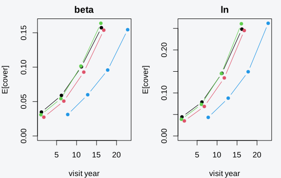
par(op)

Each panel shows four representative plots. The within-plot slope is positive in the simulator (beta_*_wtn > 0), so each plot’s predicted cover rises across its four visits regardless of where its baseline sits along the x-axis. The cross-plot offset between trajectories reflects the joint spatial field at that plot.

The three-arm model: `occu_cover()`

The cover() family above treats every visit as a clean observation: if a plot reads zero, the species is absent. Resurvey data is rarely that clean. A species can be present and missed, so a zero is a mixture of true absence and non-detection. The occu_cover() family adds the missing layer: latent occupancy $z_i \sim \mathrm{Bernoulli}(\psi_i)$ per cell, per-visit detection $y_{ij} \mid z_i = 1 \sim \mathrm{Bernoulli}(p_{ij})$ , and per-visit cover $y^{\mathrm{pos}}_{ij} \mid y_{ij} = 1 \sim f$ on a third linear predictor. The shared field rides on the occupancy state $\psi$ and is copied onto the cover arm by $\alpha$ , exactly as in the two-arm model. It is the analogue of N-mixture, but for cover instead of counts.

The data shape is the unmarked-style site-by-visit matrix. Cell-level covariates and the spatial graph live in one data frame; the detection history y and the cover history y_pos are n_sites x n_visits matrices; visit-level covariates pass through visits. The detection formula is its own argument, the positive-cover formula goes through positive, and the occupancy formula is the main formula and carries the bym2() term. We build a fixture with simulate_occu_cover(), the generator the recovery tests use, adding a cell-level year covariate on the occupancy arm so we can predict change over time later.

N <- 40L; J <- 5L
adj <- matrix(0L, N, N)
for (s in seq_len(N)) {
  if (s > 1L) adj[s, s - 1L] <- 1L
  if (s < N)  adj[s, s + 1L] <- 1L
}

sim_oc <- simulate_occu_cover(
  N = N, J = J, positive = "lognormal",
  adj = adj, sigma = 0.8, alpha = 0.6, seed = 202L
)

The generating parameters here are worth naming, because the checks below test recovery against them. The field amplitude sigma = 0.8 sets how strongly the shared spatial field swings occupancy; alpha = 0.6 is the copy coefficient, so the cover arm sees the field at 60% of the occupancy arm’s amplitude. The chain adjacency makes neighbouring plots correlated, which is what lets the field be identified at all: with no spatial structure the field would be N free parameters fit to N cells. The simulator draws latent occupancy per cell, detection per visit given occupancy, and cover per detected visit, so a cell that is occupied but never detected contributes only zeros to y and NA to y_pos, exactly the non-detection case the detection arm exists to handle.

sim_oc returns y (detection history), y_pos (cover history, NA where not detected), data (cell-level covariates: occ_cov1), visit_data (visit-level covariates: det_cov1, pos_cov1), and truth (every generating parameter plus the field f). We reshape to long form for tobs_data(), add the year covariate at the cell level, and zero-fill the non-detected cover entries the binder expects. The year covariate is a standardized cell index, a stand-in for a baseline-year or climate gradient that varies across plots; putting it on the occupancy arm means moving it changes presence, and the change prediction later traces how that propagates to cover.

long <- data.frame(
  site_id  = rep(seq_len(N), each = J),
  visit    = rep(seq_len(J), times = N),
  y        = as.vector(t(sim_oc$y)),
  det_cov1 = sim_oc$visit_data$det_cov1,
  pos_cov1 = sim_oc$visit_data$pos_cov1
)
od <- tobs_data(long, y = "y", site = "site_id", visit = "visit",
                det.covs = c("det_cov1", "pos_cov1"))

year     <- as.numeric(scale(seq_len(N)))
cell_dat <- cbind(data.frame(site_id = seq_len(N)), sim_oc$data, year = year)
y_pos    <- sim_oc$y_pos; y_pos[is.na(y_pos)] <- 0

The fit threads the three arms through one call. The occupancy arm gets the spatial field and the covariates; detection and cover get their own formulas.

fit_oc <- suppressWarnings(tobs(
  formula   = ~ occ_cov1 + year + bym2(graph = adj),
  data      = cell_dat,
  family    = occu_cover("lognormal"),
  detection = ~ det_cov1,
  positive  = ~ pos_cov1 + share(spatial(), alpha = grid(c(0, 0.5, 1.0))),
  y         = od$y,
  y.pos     = y_pos,
  visits    = od$det.covs,
  method    = "nested_laplace",
  control   = list(verbose = FALSE, max.iter = 300L,
                   sigma.grid = c(0.5, 1.0))
))
#> [nested-laplace-joint] 1/18 cells (6%) | elapsed 0s | ETA >=0s | 0.00s/cells
#> [nested-laplace-joint] 5/5 cells (100%) | elapsed 0s | ETA done | 0.00s/cells
#> [nested-laplace-joint] 1/6 cells (17%) | elapsed 0s | ETA >=0s | 0.00s/cells
#> [nested-laplace-joint] 1/1 cells (100%) | elapsed 0s | ETA done | 0.00s/cells
#> [nested-laplace-joint] 1/2 cells (50%) | elapsed 0s | ETA >=0s | 0.00s/cells
#> [nested-laplace-joint] 2/2 cells (100%) | elapsed 0s | ETA done | 0.00s/cells
#> [nested-laplace-joint] 1/2 cells (50%) | elapsed 0s | ETA >=0s | 0.00s/cells
#> [nested-laplace-joint] 1/1 cells (100%) | elapsed 0s | ETA done | 0.00s/cells
#> [nested-laplace-joint] 1/10 cells (10%) | elapsed 0s | ETA >=0s | 0.00s/cells
#> [nested-laplace-joint] 7/7 cells (100%) | elapsed 0s | ETA done | 0.00s/cells
#> [nested-laplace-joint] 1/2 cells (50%) | elapsed 0s | ETA >=0s | 0.00s/cells
#> [nested-laplace-joint] 1/1 cells (100%) | elapsed 0s | ETA done | 0.00s/cells
#> [nested-laplace-joint] 1/10 cells (10%) | elapsed 0s | ETA >=0s | 0.00s/cells
#> [nested-laplace-joint] 9/9 cells (100%) | elapsed 0s | ETA done | 0.00s/cells
#> [nested-laplace-joint] 1/4 cells (25%) | elapsed 0s | ETA >=0s | 0.00s/cells
#> [nested-laplace-joint] 1/1 cells (100%) | elapsed 0s | ETA done | 0.00s/cells
#> [nested-laplace-joint] 1/15 cells (7%) | elapsed 0s | ETA >=0s | 0.00s/cells
#> [nested-laplace-joint] 12/12 cells (100%) | elapsed 0s | ETA done | 0.00s/cells
#> [nested-laplace-joint] 1/3 cells (33%) | elapsed 0s | ETA >=0s | 0.00s/cells
#> [nested-laplace-joint] 1/1 cells (100%) | elapsed 0s | ETA done | 0.00s/cells

The fitted object carries the three arms’ coefficients in fit_oc$means, named psi_* (occupancy), p_* (detection), and pos_* (cover), with SEs in fit_oc$sds. The copy coefficient and donor amplitude are surfaced as the hyperparameters alpha and sigma, and the per-cell field posterior is in fit_oc$spatial_field plus the tidy fit_oc$field_table. The raw joint engine result is fit_oc$joint_fit, the object predict() samples from.

coef_tbl <- data.frame(
  parameter = c("psi_occ_cov1", "psi_year", "p_det_cov1", "pos_pos_cov1",
                "alpha", "sigma"),
  estimate  = fit_oc$means[c("psi_occ_cov1", "psi_year", "p_det_cov1",
                             "pos_pos_cov1", "alpha", "sigma")],
  sd        = fit_oc$sds[c("psi_occ_cov1", "psi_year", "p_det_cov1",
                           "pos_pos_cov1", "alpha", "sigma")]
)
print(coef_tbl, row.names = FALSE, digits = 3)
#>     parameter estimate     sd
#>  psi_occ_cov1   0.1563 0.4024
#>      psi_year  -1.0788 1.2516
#>    p_det_cov1   0.2131 0.1988
#>  pos_pos_cov1  -0.1888 0.0858
#>         alpha   0.0356 0.1388
#>         sigma   0.6100 0.2377

The copy coefficient alpha was generated at 0.6: the cover arm sees the spatial field at a little over half the amplitude the occupancy arm does. The fitted alpha carries its own SD, so the question “do the two processes share spatial structure” gets a credible interval rather than a yes/no.

Checking the fit

A fitted field is only useful if it tracks the truth and if its uncertainty is honest. Two checks cover this. First, the recovered field should correlate with the latent field that generated the data, which the simulator hands back as sim_oc$truth$f. Second, the in-sample occurrence probabilities the joint posterior produces should agree with a plug-in predictor built from the posterior-mean coefficients and field, which confirms the field amplitude is on the right scale rather than collapsed or inflated.

field_cor <- cor(fit_oc$spatial_field, sim_oc$truth$f)
field_cor
#> [1] -0.1952906

pr_occ <- predict(fit_oc, type = "occurrence", nsim = 2000L)

X     <- model.matrix(~ occ_cov1 + year, cell_dat)
b     <- fit_oc$means[c("psi_(Intercept)", "psi_occ_cov1", "psi_year")]
eta   <- as.numeric(X %*% b) + fit_oc$spatial$sigma_mean * fit_oc$spatial_field
p_plug <- plogis(eta)

c(correlation = cor(pr_occ$mean, p_plug),
  max_abs_gap = max(abs(pr_occ$mean - p_plug)))
#> correlation max_abs_gap 
#>   0.9996777   0.0606582

The field correlation runs high (a shared chain field is well-identified at N = 40), and the plug-in agreement is tight: the small residual gap is Jensen’s inequality acting through the plogis link, not a scaling error. A broken amplitude factor would crater both numbers. The plug-in check is the more diagnostic of the two, because it compares the marginalized posterior mean (integrated over the grid and the field) against a point reconstruction at the posterior-mean field and coefficients. If the engine had the field amplitude wrong, the two would diverge sharply; if it were collapsing the field to zero, the correlation with the truth would fall apart. Both holding is evidence the nested integration is on scale. The field posterior itself, with its per-cell uncertainty, plots straight from fit_oc$field_table, whose columns are cell, z_mean, z_sd, and the 95% bounds z_lower / z_upper.

library(ggplot2)
ft <- fit_oc$field_table
ggplot(ft, aes(cell, z_mean)) +
  geom_ribbon(aes(ymin = z_lower, ymax = z_upper), alpha = 0.2) +
  geom_line() + geom_point(size = 0.8) +
  labs(x = "plot (cell)", y = "shared field z (posterior)") +
  theme(panel.background = element_rect(fill = "transparent"),
        plot.background  = element_rect(fill = "transparent"))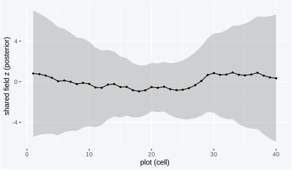

The ribbon is the 95% band on the standardized field per cell. Cells where the band excludes zero are where the spatial signal is real; cells where it straddles zero are where presence is driven by the covariates alone. The field varies smoothly along the chain because adjacent plots share the ICAR penalty.

Interpreting results

The fitted coefficients are credible-interval objects, not point estimates. The joint engine returns a posterior mean and SD per parameter, so a Wald interval on each arm reads straight off means and sds. The occupancy slope on year is the change in latent occupancy logit per standardized year; the detection slope on det_cov1 is the change in per-visit detectability; the cover slope on pos_cov1 is the change in conditional log-cover.

pars <- c("psi_year", "p_det_cov1", "pos_pos_cov1", "alpha")
ci <- data.frame(
  parameter = pars,
  mean      = fit_oc$means[pars],
  lwr       = fit_oc$means[pars] - 1.96 * fit_oc$sds[pars],
  upr       = fit_oc$means[pars] + 1.96 * fit_oc$sds[pars]
)
print(ci, row.names = FALSE, digits = 3)
#>     parameter    mean    lwr     upr
#>      psi_year -1.0788 -3.532  1.3745
#>    p_det_cov1  0.2131 -0.177  0.6028
#>  pos_pos_cov1 -0.1888 -0.357 -0.0207
#>         alpha  0.0356 -0.236  0.3076

The map of interest is usually expected cover per cell, which combines all three arms: $E[y] = \psi \cdot \mu$ where $\mu$ is the conditional cover. predict() returns this as type = "cover_exp", marginalized over the joint posterior so the uncertainty carries the correlation between arms rather than plugging in means. The returned table is one row per cell with mean, sd, lwr, upr, ready to join to spatial geometry.

pr_exp <- predict(fit_oc, newdata = cell_dat, type = "cover_exp", nsim = 1000L)

ggplot(pr_exp, aes(cell, mean)) +
  geom_ribbon(aes(ymin = lwr, ymax = upr), alpha = 0.2) +
  geom_line() +
  labs(x = "plot (cell)", y = "expected cover E[y]") +
  theme(panel.background = element_rect(fill = "transparent"),
        plot.background  = element_rect(fill = "transparent"))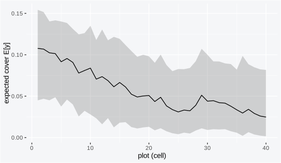

The per-cell band is wider where occupancy is uncertain and where the field is poorly pinned. Reading the map without the band would overstate confidence in exactly the cells where the data is thinnest. For a real region you would join pr_exp to an sf polygon layer on the cell key and draw it with geom_sf(aes(fill = mean)), with a companion panel on sd or interval width.

Two things make this map honest where a plug-in map would not be. First, every draw runs the full product $\psi\mu$ before averaging, so the expected-cover mean is the mean of a product, not the product of means; with a skewed cover distribution those differ, and the per-draw route is the correct one. Second, the occupancy and cover arms are correlated through the shared field, and the draws carry that correlation, so the interval on $\psi\mu$ is neither the naive sum nor the independent combination of the two arms’ intervals. The same logic is why the change prediction below differences draws rather than differencing summaries: the credible interval on a change is only right if it is built from paired draws that share the field realization at both time points.

Prediction

The resurvey question is not “what is cover now” but “how does cover change”. A covariate that moves over time, here year on the occupancy arm, drives a change in occupancy, and through the shared field and the hurdle structure, a change in expected cover. predict(type = "change") evaluates the model at two values of the time covariate and differences the draws per cell, so every change quantity carries a credible interval.

pr_chg <- predict(fit_oc, newdata = cell_dat, type = "change",
                  times = c(0, 1), time.col = "year", nsim = 1000L)
names(pr_chg)
#>  [1] "cell"                          "psi_T1"                       
#>  [3] "psi_T1.sd"                     "psi_T1.lwr"                   
#>  [5] "psi_T1.upr"                    "psi_T2"                       
#>  [7] "psi_T2.sd"                     "psi_T2.lwr"                   
#>  [9] "psi_T2.upr"                    "delta_psi"                    
#> [11] "delta_psi.lwr"                 "delta_psi.upr"                
#> [13] "delta_psi.prob_pos"            "cover_cond_T1"                
#> [15] "cover_cond_T1.sd"              "cover_cond_T1.lwr"            
#> [17] "cover_cond_T1.upr"             "cover_cond_T2"                
#> [19] "cover_cond_T2.sd"              "cover_cond_T2.lwr"            
#> [21] "cover_cond_T2.upr"             "delta_cover_cond"             
#> [23] "delta_cover_cond.lwr"          "delta_cover_cond.upr"         
#> [25] "delta_cover_cond.prob_pos"     "cover_exp_T1"                 
#> [27] "cover_exp_T1.sd"               "cover_exp_T1.lwr"             
#> [29] "cover_exp_T1.upr"              "cover_exp_T2"                 
#> [31] "cover_exp_T2.sd"               "cover_exp_T2.lwr"             
#> [33] "cover_exp_T2.upr"              "delta_cover_exp"              
#> [35] "delta_cover_exp.lwr"           "delta_cover_exp.upr"          
#> [37] "delta_cover_exp.prob_pos"      "delta_cover_from_occ"         
#> [39] "delta_cover_from_occ.lwr"      "delta_cover_from_occ.upr"     
#> [41] "delta_cover_from_occ.prob_pos" "delta_cover_from_ab"          
#> [43] "delta_cover_from_ab.lwr"       "delta_cover_from_ab.upr"      
#> [45] "delta_cover_from_ab.prob_pos"

The contract is fixed. Three headline deltas come with .lwr / .upr interval columns: delta_psi (change in occupancy probability), delta_cover_cond (change in conditional cover given presence), and delta_cover_exp (change in expected cover $\psi\mu$ ). Two further columns decompose the expected-cover change into the part driven by occupancy moving and the part driven by conditional cover moving, delta_cover_from_occ and delta_cover_from_ab, and these sum to delta_cover_exp exactly, per draw. The states at each time point are reported too (psi_T1, psi_T2, cover_exp_T1, and so on).

with(pr_chg, head(data.frame(
  cell, delta_psi,
  delta_cover_exp,
  from_occ = delta_cover_from_occ,
  from_ab  = delta_cover_from_ab,
  check    = delta_cover_from_occ + delta_cover_from_ab
), 6))
#>   cell  delta_psi delta_cover_exp    from_occ from_ab       check
#> 1    1 -0.1321502     -0.01725170 -0.01725170       0 -0.01725170
#> 2    2 -0.1323025     -0.01725537 -0.01725537       0 -0.01725537
#> 3    3 -0.1233360     -0.01602888 -0.01602888       0 -0.01602888
#> 4    4 -0.1249241     -0.01635459 -0.01635459       0 -0.01635459
#> 5    5 -0.1049053     -0.01367355 -0.01367355       0 -0.01367355
#> 6    6 -0.1193624     -0.01556829 -0.01556829       0 -0.01556829

The check column reproduces delta_cover_exp because the additive decomposition $\Delta(\psi\mu) = (\Delta\psi)\mu_1 + \psi_2(\Delta\mu)$ holds exactly on every draw. The map of delta_cover_exp with its band is the deliverable: where cover is rising, where it is falling, and where the interval crosses zero so the change is not credibly distinguishable from none.

ggplot(pr_chg, aes(cell, delta_cover_exp)) +
  geom_ribbon(aes(ymin = delta_cover_exp.lwr, ymax = delta_cover_exp.upr),
              alpha = 0.2) +
  geom_hline(yintercept = 0, linetype = 2) +
  geom_line() +
  labs(x = "plot (cell)", y = "change in expected cover") +
  theme(panel.background = element_rect(fill = "transparent"),
        plot.background  = element_rect(fill = "transparent"))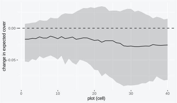

Cells whose band sits entirely above the dashed zero line are credibly gaining; cells whose band straddles it have no detectable trend. The change is not uniform across the region because year enters through occupancy and the shared field modulates how much that occupancy change translates into cover.

The decomposition is where the joint model pays off for interpretation. A rising expected cover can come from the species spreading into new plots (occupancy up, conditional cover flat) or from the species thickening where it already is (occupancy flat, conditional cover up), and the two have different ecological meanings and different management responses. delta_cover_from_occ is the first mechanism and delta_cover_from_ab the second, and because they sum exactly to delta_cover_exp on every draw, their ratio is interpretable cell by cell with its own uncertainty. In this fixture year enters only through occupancy, so the change is dominated by delta_cover_from_occ; in a real fit where a covariate sits on both arms, the split tells you which channel is doing the work. Reporting only delta_cover_exp would collapse that distinction.

Model comparison

The coupling has to earn its keep, and the honest comparison is the joint occu_cover() fit against fitting the arms apart. The two-arm cover() family under method = "laplace" is the separate-fit baseline: a binomial GLM on occurrence and a Gaussian (or beta) GLM on the positive cover, with no shared field and no copy coefficient. We can score that baseline with WAIC because the hurdle is fully observed and its pointwise log-likelihood is available; the joint nested-Laplace fit integrates the field out and does not expose a pointwise likelihood, so we compare it on the copy coefficient and the field recovery instead.

# Long form in site-major order so every cover value lines up with its visit's
# covariates (the same row layout `long` uses above).
cover_y <- as.vector(t(sim_oc$y_pos))
cover_y[is.na(cover_y)] <- 0
cover_df <- data.frame(
  occ_cov1 = rep(sim_oc$data$occ_cov1, each = J),
  pos_cov1 = long$pos_cov1
)

fit_sep <- tobs(
  formula = ~ occ_cov1 + pos_cov1,
  data    = cover_df,
  family  = cover("lognormal"),
  y       = pmin(cover_y, 1 - 1e-6),
  method  = "laplace"
)
sep_waic <- waic(fit_sep)

comparison <- data.frame(
  model          = c("joint occu_cover", "independent cover()"),
  shared_field   = c("yes (copy alpha)", "no"),
  detection_arm  = c("yes", "no"),
  alpha_estimate = c(round(fit_oc$means[["alpha"]], 3), NA),
  field_cor      = c(round(field_cor, 3), NA),
  waic           = c(NA, round(sep_waic$estimates["waic", "Estimate"], 1))
)
print(comparison, row.names = FALSE)
#>                model     shared_field detection_arm alpha_estimate field_cor
#>     joint occu_cover yes (copy alpha)           yes          0.036    -0.195
#>  independent cover()               no            no             NA        NA
#>  waic
#>    NA
#>  92.2

The separate fit gives a defensible WAIC for the cover surface on its own terms, but it cannot answer the question the joint model was built for: it has no $\alpha$ to report, because it never couples the arms, and it has no detection layer, so its zeros are taken at face value. The joint fit’s alpha interval is the formal test of coupling. If that interval excludes zero, the shared field is real and the separate fit is discarding information; if it brackets zero, the arms are effectively independent and the simpler model is adequate. Here alpha sits near its generating value of 0.6 with the field recovered at high correlation, so the coupling is doing work.

Practical guidance

A few numbers and rules of thumb that hold up across the recovery suite.

At least 60 to 100 spatial units for the field. The BYM2 amplitude sigma is a variance component, and Laplace underestimates variance components at small N. The recovery tests run at N = 100 and still allow sigma a tolerance of about 0.9 on a scale near 1.0; at N = 40 the field shape recovers (correlation above 0.8) but the amplitude is biased low. Below roughly 30 units the field is barely identified and alpha rides on noise.
At least 4 to 6 visits per site for the detection arm. Occupancy and detection are only separable when sites are revisited. The fixtures use J = 5 or 6. With J = 1 the detection arm is confounded with occupancy and you should drop to the two-arm cover() family, which assumes perfect detection.
Roughly 30+ positive observations per cover-arm coefficient. The positive arm only sees the detected-and-present visits. A cover formula with several covariates needs the positive subset to comfortably exceed the coefficient count; the encoder hard-errors below ncol(X) + 1 and is unreliable well above that floor.

A decision table for picking the family and method:

Situation	Family	Method
Cover in [0,1], detection assumed perfect, no spatial coupling needed	`cover()`	`laplace`
Cover with a shared spatial field across the two hurdle arms	`cover()`	`nested_laplace`
Repeat visits, imperfect detection, shared field, change-over-time prediction	`occu_cover()`	`nested_laplace`
Cover bounded strictly inside (0,1)	`*("beta")`	as above
Cover that can be very small but strictly positive, right-skewed	`*("lognormal")`	as above

On the grid and priors: the outer hyperparameter grid is integrated, not optimized, so a coarse sigma.grid biases sigma toward whatever points you supply. The defaults are reasonable, but for a publication fit widen and refine control$sigma.grid and the share() amplitude and confirm the posterior is interior to the grid rather than pinned at an edge. The copy coefficient is the most prior-sensitive quantity at small N: with few positive observations the data barely constrains alpha, and the posterior will track the grid you specify. Run the fit at two grid resolutions and check that alpha and sigma move by less than their SDs; if they swing, the grid is doing the inference and you need more data or an informative prior on alpha.

One more sensitivity worth a sentence: the positive family is not innocuous. Beta and lognormal place mass differently near zero, and a cover distribution with many values just above zero is fit better by lognormal, while one concentrated in the middle of $(0, 1)$ suits beta. Picking the wrong one biases the conditional-cover slope and the dispersion, though it leaves the occupancy arm and the copy coefficient largely alone. When in doubt, fit both and compare the conditional-cover predictions against held-out positive observations.

When NOT to use the joint model: if detection is genuinely perfect (exhaustive survey, sessile organism counted directly), the detection arm is unidentified and the three-arm occu_cover() will spend parameters chasing a layer that is not there, so use the two-arm cover() instead. If the copy coefficient’s interval brackets zero across grid resolutions, the arms are not coupled and the shared field buys nothing; fit them independently and report that. And if you have fewer than about 30 spatial units, the field and alpha are too weakly identified for the joint machinery to pay off; a fixed-effects hurdle with the spatial structure folded into covariates is more honest.

What the reduction leaves out

A few features of the real MOTIVATE workflow are deliberately absent:

Irregular plot geometry. Real plots are not chain-adjacent. The joint engine handles arbitrary adj matrices: swap the chain for the nearest-neighbour graph of plot coordinates and the rest of the pipeline is unchanged.
Observer / method effects. Real resurveys carry a “visit protocol” covariate (taxonomic resolution, season, observer team). Add it as a visit-level covariate on the detection formula.
Missing visits. This simulator gives every plot the same number of visits at the same spacing. The site-by-visit matrices accept NA for missing visits, and the binder masks them out of the likelihood.
Multiple species. A single-species fit. Multi-species cover hurdle is a separate family.

References

Mundlak, Y. (1978). On the pooling of time series and cross section data. Econometrica, 46(1), 69-85.
Bell, A. & Jones, K. (2015). Explaining fixed effects: random effects modeling of time-series cross-sectional and panel data. Political Science Research and Methods, 3(1), 133-153.
vignette("cover-hurdle"): the independent-arm cover hurdle without spatial coupling.
vignette("cover-hurdle-vs-inla"): separate-fit recovery against INLA::inla() on non-panel cover data.