29  R internals

What, exactly, is a vector?

You have written thousands of them by now, filtered them, mapped functions over them, watched them copy themselves at surprising moments. But the object itself, the thing sitting in memory when you type x <- c(1, 2, 3), has remained invisible. This chapter opens it up. We are going to look at the C structs that R allocates on the heap, the pointer arithmetic that makes vectorized operations fast, the reference counter that decides when copies happen, and the garbage collector that reclaims everything you abandon. None of this is necessary for writing good R. But it makes the design choices you have seen throughout this book (copy-on-modify, lazy evaluation, lexical scoping) feel less like arbitrary rules and more like consequences of a single engineering blueprint.

R’s C implementation descends from S, which John Chambers created at Bell Labs in the 1970s. When Ross Ihaka and Robert Gentleman reimplemented it at the University of Auckland in the early 1990s, they borrowed the evaluation model from Scheme and dressed it in S-compatible syntax. The linked-list environments come from Lisp; the vectorized operations come from S; the garbage collector is a textbook generational mark-and-sweep. What holds all of it together is a single data structure.

29.1 Stack and heap

A running program has two regions of memory. The stack is small, fast, and automatic: when you call a function, its local variables go on the stack, and when the function returns, they vanish. The heap is large, slow, and manual: objects allocated on the heap survive until something explicitly frees them (in C) or until a garbage collector determines that nothing points to them anymore (in R, Python, Java). Every R object lives on the heap. When you write x <- c(1, 2, 3), R allocates a block of memory on the heap, fills it with your three numbers, and stores a pointer to that block in the binding for x. When x goes out of scope and nothing else references it, R’s garbage collector reclaims the memory. The stack holds the bookkeeping (which function called which, where to return); the heap holds the data.

29.2 Every object is a SEXP

In R’s C source code, every R object, without exception, is represented as a SEXP: a pointer to a SEXPREC struct. The name stands for “S expression,” inherited from Lisp. When you write x <- c(1, 2, 3), R allocates a SEXPREC on the heap, fills it with the data for a three-element numeric vector, and stores the pointer in the binding for x.

The SEXPREC struct has two parts. The header is the same for every object, and it contains:

• A type tag (SEXPTYPE): an integer identifying what kind of object this is (integer vector, closure, environment, etc.).
• GC information: flags the garbage collector uses to track whether the object is reachable.
• Reference count: how many names point to this object (used to decide whether copy-on-modify needs to copy).
• Attributes: a pointer to a pairlist of attributes (names, class, dim, etc.).

The payload varies by type. For a numeric vector, it is a contiguous block of C double values. For a closure, it is three pointers (formals, body, environment). For an environment, it is a hash table plus a pointer to the parent environment. So every R object, from a humble integer to a deeply nested list of data frames, wears the same uniform; only the payload inside differs.

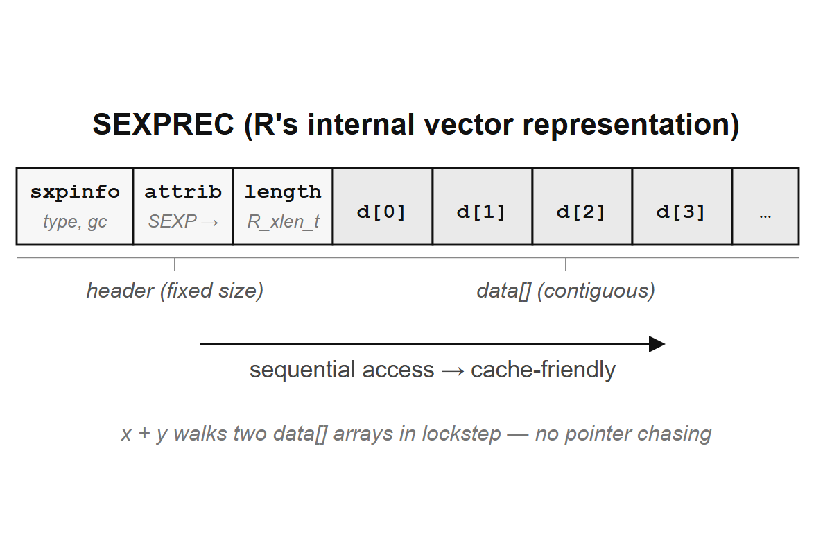
Figure 29.1: The SEXPREC struct: a fixed-size header followed by a contiguous data array. x + y walks two arrays in lockstep with no pointer chasing.

You can see the type tag from R with typeof():

typeof(1:5)
#> [1] "integer"
typeof(c(1.0, 2.0))
#> [1] "double"
typeof("hello")
#> [1] "character"
typeof(list(1, 2))
#> [1] "list"
typeof(sum)
#> [1] "builtin"
typeof(mean)
#> [1] "closure"

typeof() returns the SEXPTYPE name as a string. The mapping between R concepts and SEXPTYPEs is direct:

R concept	SEXPTYPE	C constant
Integer vector	integer	INTSXP
Double vector	double	REALSXP
Character vector	character	STRSXP
Logical vector	logical	LGLSXP
List	list	VECSXP
Function (closure)	closure	CLOSXP
Built-in function	builtin	BUILTINSXP
Special function	special	SPECIALSXP
Environment	environment	ENVSXP
Promise	promise	PROMSXP
Language object	language	LANGSXP
Symbol (name)	symbol	SYMSXP

Some of these are familiar. CLOSXP is the closure from Section 18.4. ENVSXP is the environment from Section 18.1. PROMSXP is the promise from Chapter 23. The new ones, LANGSXP and SYMSXP, are the building blocks of R’s metaprogramming system (Chapter 26), and we will meet them properly there.

Notice that sum and mean have different types. sum is a builtin, implemented directly in C, evaluating all its arguments before being called. mean is a closure, a regular R function with formals, a body, and an environment. The distinction matters at the C level but rarely at the R level. What matters at both levels is being able to see inside these objects, so how do you look?

29.3 Inspecting objects

R provides a hidden function, .Internal(inspect()), that dumps the raw C-level representation of any object:

x <- c(1.5, 2.5, 3.5)
.Internal(inspect(x))
#> @0x000001ef8123bbd8 14 REALSXP g0c3 [REF(2)] (len=3, tl=0) 1.5,2.5,3.5

The output shows the memory address, the SEXPTYPE (REALSXP), the reference count, and the actual data values. Terse, but informative.

The lobstr package provides friendlier inspection tools:

library(lobstr)

obj_addr(x)
#> [1] "0x1ef8123bbd8"
obj_size(x)
#> 80 B

obj_addr() returns the memory address as a string. obj_size() reports total memory consumption, including the header, so for a three-element numeric vector you get the SEXPREC header (approximately 64 bytes, implementation-dependent) plus three times 8 bytes for the doubles, plus some alignment padding.

Where things get interesting is ref(), which shows whether two names point to the same underlying object:

y <- x
ref(x, y)
#> [1:0x1ef8123bbd8] <dbl> 
#>  
#> [1:0x1ef8123bbd8]

Both x and y point to the same memory address. No copy has been made. This is the copy-on-modify mechanism you saw in Section 9.4, now visible at the pointer level.

y[1] <- 99
ref(x, y)
#> [1:0x1ef8123bbd8] <dbl> 
#>  
#> [2:0x1ef7f226fa8] <dbl>

After modification, y points to a different address. R copied the vector when y was modified, because x still needed the original. The copy decision depends on how many names point to the same data, which raises the obvious question: how does R keep track?

Exercises

1. Use typeof() to check the type of: TRUE, 1L, 1.0, 1+2i, raw(1), quote(x + 1), as.name("x"). Which ones surprise you?

2. Run .Internal(inspect(list(1, "a", TRUE))). How many SEXPs do you see? Why more than one?

3. Create a <- 1:1e6 and b <- a. Check with lobstr::ref() that they share the same address. Now do b[1] <- 0L. Do they still share? What does lobstr::obj_size(a, b) report?

29.4 Memory layout of vectors

A numeric vector in R is stored as a SEXPREC header followed by a contiguous block of C double values, and “contiguous” is the word that matters here: the doubles sit next to each other in memory, with no gaps or pointers between them, exactly like a C array or a NumPy array.

/* Simplified layout of a REALSXP (not actual R source) */
struct SEXPREC {
    /* header: type, gc flags, refcount, attributes, ... */
    sxpinfo_struct sxpinfo;
    SEXP attrib;
    SEXP gengc_next_node;
    SEXP gengc_prev_node;
    /* payload for vectors: */
    R_xlen_t length;
    R_xlen_t truelength;
    double data[];  /* flexible array member: the actual numbers */
};

The contiguous layout is why vectorized operations are fast. When R computes x + y, the C code walks two arrays of doubles in lockstep, reading from sequential memory addresses; modern CPUs are optimized for exactly this access pattern, with hardware prefetchers loading the next cache line before you need it and SIMD instructions adding multiple doubles in a single clock cycle.

An integer vector (INTSXP) has the same layout but with int instead of double. A logical vector (LGLSXP) also uses int (not char), which is why logicals take 4 bytes per element, not 1.

Character vectors are a different beast entirely. A STRSXP is a vector of pointers to CHARSXP objects, where each CHARSXP holds an immutable C string. R interns (deduplicates) these strings globally, so two identical strings share the same CHARSXP:

a <- "hello"
b <- "hello"
.Internal(inspect(a))
#> @0x000001ef7f525c08 16 STRSXP g0c1 [REF(5)] (len=1, tl=0)
#>   @0x000001ef7f0869a8 09 CHARSXP g0c1 [MARK,REF(4),gp=0x60] [ASCII] [cached] "hello"
.Internal(inspect(b))
#> @0x000001ef7f525498 16 STRSXP g0c1 [REF(5)] (len=1, tl=0)
#>   @0x000001ef7f0869a8 09 CHARSXP g0c1 [MARK,REF(4),gp=0x60] [ASCII] [cached] "hello"

The outer STRSXP addresses differ (they are separate character vectors), but the inner CHARSXP they point to is the same object. This interning saves memory when the same strings appear repeatedly, as in a factor or a character column with many repeated levels.

A list (VECSXP) is a vector of SEXP pointers. Each element can point to any R object of any type, which is why lists are heterogeneous: the list itself is just an array of pointers, and the pointed-to objects can be anything. This pointer-based layout has consequences for how R handles tabular data.

Data frames and cache friendliness. A data frame is a list of column vectors, and each column is a contiguous array. Operations that scan down a column (summing, filtering, grouping) touch sequential memory and benefit from cache prefetching. Operations that scan across rows jump between columns, touching non-sequential addresses and thrashing the cache. This is why column-wise operations in R are generally faster than row-wise ones, and why apply(df, 1, f) (row-wise) is slower than lapply(df, f) (column-wise). But memory layout only tells half the story; the other half is what happens when two names share the same layout.

Exercises

1. Use lobstr::obj_size() to compare the size of integer(1000) and double(1000). Is the ratio exactly 1:2? Why or why not?

2. Create two character vectors: x <- rep("abcdef", 1000) and y <- paste0("abcdef", seq_len(1000)). Compare their sizes with obj_size(). Why is x much smaller?

3. Why does object.size(data.frame(a = 1:1e6)) report less memory than object.size(data.frame(a = as.double(1:1e6)))?

29.5 Reference counting and copy-on-modify

In Section 9.4, you learned that R copies objects only when they are modified and shared. But how does R decide?

Every SEXPREC header contains a reference count: the number of names (bindings) currently pointing to this object. When you assign y <- x, R increments the reference count on the underlying object instead of copying it. When you modify y, R checks the count: if it is 1 (only y points to the object), R can modify in place; if it is greater than 1, R must copy first.

x <- c(1, 2, 3)
.Internal(inspect(x))
#> @0x000001ef8039eb48 14 REALSXP g0c3 [REF(2)] (len=3, tl=0) 1,2,3

The [MARK,NAM(X)] in the inspect output shows the reference count. (The exact format varies by R version.)

y <- x
.Internal(inspect(x))
#> @0x000001ef8039eb48 14 REALSXP g0c3 [REF(5)] (len=3, tl=0) 1,2,3

After y <- x, the reference count increases but the address stays the same. Both names share the same data.

Historical note: the NAMED mechanism. Before R 4.0, R used a cruder system called NAMED, with only three states: 0 (no references), 1 (one reference), and 2 (multiple references, or “we have lost count”). The problem was that NAMED could never decrease; once an object reached NAMED=2, R always copied it on modification, even if one reference had long since disappeared. The current reference counting system, introduced by Luke Tierney, tracks actual counts and can decrease them when bindings are removed, eliminating a whole class of unnecessary copies.

You can observe the practical effect. Modifying a vector inside a function that receives it as an argument triggers a copy, because the caller’s binding and the function’s parameter both point to the object (reference count of at least 2):

f <- function(v) {
  v[1] <- 0
  v
}

x <- c(1, 2, 3)
y <- f(x)
ref(x, y)
#> [1:0x1ef8146ea48] <dbl> 
#>  
#> [2:0x1ef8146e048] <dbl>

x and y are different objects. The copy happened inside f when v[1] <- 0 was executed, because v shared its data with x.

TipOpinion

Reference counting is why you should not worry too much about “R copies everything.” R copies only when it must: when an object is shared and you modify it. Patterns that look wasteful, like passing large data frames into functions, are often free, because the function receives a pointer, not a copy. The copy happens only if the function modifies the data, which idiomatic functional code rarely does.

Exercises

1. Predict whether a copy occurs in each case, then verify with lobstr::ref():

   a <- 1:1e6
   b <- a           # copy?
   b[1] <- 0L       # copy?
   c <- a            # copy?
   rm(a)
   c[1] <- 0L       # copy now?

2. Write a function that takes a vector, does not modify it, and returns its obj_addr(). Call it with a large vector. Is the address the same inside and outside the function?

29.6 Garbage collection

Objects get created; reference counts rise and fall; eventually some objects have no references at all. What happens to them?

R uses a tracing garbage collector with a mark-and-sweep algorithm. When R runs low on memory, the collector pauses execution, traces all reachable objects by following pointers from the known roots (the global environment, the call stack, the symbol table), marks them, and sweeps away everything unmarked. If a SEXP has no path back to any root, it ceases to exist.

The collector is generational, dividing objects into three generations based on how long they have survived. New objects are generation 0; objects that survive one collection get promoted to generation 1, then to generation 2. The insight behind this design is that most objects die young (temporary vectors in a loop, intermediate results in a pipeline), so collecting generation 0 frequently and generation 2 rarely is efficient. It is the same principle behind most modern garbage collectors, from Java’s G1 to Go’s concurrent collector.

You can trigger collection manually and see the results:

gc()
#>           used (Mb) gc trigger (Mb) max used (Mb)
#> Ncells  683323 36.5    1417982 75.8  1417982 75.8
#> Vcells 1253621  9.6    8388608 64.0  1932447 14.8

The output shows memory usage in Ncells (cons cells, used for pairlists and language objects) and Vcells (vector cells, used for vector data). The “used” column is current consumption; “max used” is the peak since the last gc(reset = TRUE).

gcinfo(TRUE) tells R to print a message every time the garbage collector runs, which is noisy but revealing when you want to understand how much allocation a piece of code is doing:

gcinfo(TRUE)
x <- lapply(1:1000, function(i) rnorm(1000))
gcinfo(FALSE)

PROTECT and UNPROTECT at C level. If you write C code that creates R objects (via .Call()), you must tell the garbage collector about them. The collector can run at any allocation point, and if your newly created SEXP is not reachable from any root, it will be swept away while you are still using it. The PROTECT() macro adds an object to a protection stack; UNPROTECT(n) removes the last n entries. Forgetting to PROTECT is the single most common source of bugs in R’s C extensions: intermittent segfaults that depend on the exact moment the GC happens to run, which means they almost never reproduce on the developer’s machine and almost always reproduce in production.

/* Example: a C function callable from R via .Call() */
SEXP add_one(SEXP x) {
    SEXP result = PROTECT(allocVector(REALSXP, length(x)));
    double *px = REAL(x);
    double *pr = REAL(result);
    for (R_xlen_t i = 0; i < length(x); i++) {
        pr[i] = px[i] + 1.0;
    }
    UNPROTECT(1);
    return result;
}

The PROTECT(allocVector(...)) call allocates a new vector and protects it in a single line. The UNPROTECT(1) at the end removes it from the protection stack just before returning. Between those two points, the GC knows not to collect result. Get the count wrong, and you get either a segfault or a stack overflow, which is exactly why higher-level interfaces like Rcpp exist.

Exercises

1. Run gc() and note the “used” Vcells. Then create x <- rnorm(1e7), run gc() again, and note the change. Now rm(x) and gc() one more time. Did the Vcells return to roughly the original level?

2. What does gc(full = TRUE) do differently from gc()?

3. In the C function add_one above, what would happen if you removed the PROTECT() call? Would the bug appear every time, or only sometimes?

29.7 The evaluator

R is an interpreted language, which means something very specific: when you type an expression at the console, R parses it into an internal tree structure (a LANGSXP), then walks that tree in a function called eval() in the file eval.c. There is no compilation step, no bytecode (well, there is a bytecode compiler now, but the default path is interpretation), just a C function recursively walking a tree of SEXPs.

The core of eval() is a large switch statement on the SEXPTYPE of the expression:

/* Simplified sketch of eval.c (not actual code) */
SEXP eval(SEXP e, SEXP rho) {
    switch (TYPEOF(e)) {
    case SYMSXP:    /* symbol: look up in environment */
        return findVar(e, rho);
    case LANGSXP:   /* function call: evaluate function and args, then apply */
        return applyClosure(e, rho);
    case PROMSXP:   /* promise: force it */
        return forcePromise(e);
    case REALSXP:
    case INTSXP:
    case STRSXP:    /* self-evaluating literals */
        return e;
    /* ... many more cases ... */
    }
}

When the expression is a symbol (SYMSXP), the evaluator looks it up in the environment rho by walking the chain of parent environments. When it is a function call (LANGSXP), the evaluator finds the function, evaluates the arguments (wrapping them in promises for closures), and calls it. When it is a literal (a number, a string), it returns the value unchanged.

This is why R is slower than compiled languages for tight loops: every iteration goes through this switch statement, every variable access is an environment lookup, and every function call involves promise creation and argument matching. Vectorized code avoids most of this overhead by dropping into C for the inner loop, where none of these costs exist. But the environments that the evaluator searches through are themselves data structures worth understanding.

Environments as linked frames. An environment in R is a hash table of bindings (name-to-SEXP mappings) plus a pointer to a parent environment. Variable lookup walks the chain: check the current environment’s hash table, then the parent’s, then the grandparent’s, up to the global environment and then the search path of attached packages. The hash table uses a simple chaining scheme, and small environments (fewer than about 5 bindings) skip the hash table entirely, using linear search through a pairlist instead, because the overhead of hashing is not worth it for tiny frames.

29.8 Promises at C level

In Chapter 23, you learned that function arguments are wrapped in promises. Here is what a promise actually looks like in memory.

At the C level, a promise (PROMSXP) is a struct with three fields:

1. Expression (PRCODE): the unevaluated expression, stored as a LANGSXP or SYMSXP.
2. Environment (PRENV): the environment where the expression should be evaluated.
3. Value (PRVALUE): initially R_UnboundValue (a sentinel). After the promise is forced, this holds the cached result.

When the evaluator encounters a PROMSXP, it checks PRVALUE. If it is still R_UnboundValue, it evaluates PRCODE in PRENV, stores the result in PRVALUE, and sets PRENV to R_NilValue (allowing the original environment to be garbage collected). If PRVALUE is already set, it returns the cached value immediately. Evaluate once, cache forever.

This three-field structure explains several behaviors you have seen:

• Default arguments that refer to other arguments work because the promise’s environment is the function’s execution environment, where earlier parameters are already bound.
• substitute() can extract the unevaluated expression because it reads PRCODE without forcing the promise.
• The lazy evaluation trap in function factories (Section 20.2) happens because the promise captures the expression and the environment at call time, but evaluates them later, when the environment may have changed.

You cannot inspect promises from R without forcing them — a fundamental property of the design, not an oversight:

f <- function(x) {
  # This LOOKS like it checks the type before forcing, but typeof(x)
  # itself forces the promise. By the time cat() prints, x is already
  # evaluated. There is no way around this in R.
  cat("typeof x:", typeof(x), "\n")
  x
}
f(1 + 1)
#> typeof x: double
#> [1] 2

If R provided a way to get the type without forcing, you would see "promise". But calling typeof(x) is itself an access of x, which forces the promise, so by the time the result is printed, x is already "double". The promise is deliberately invisible from R’s perspective: any inspection forces evaluation, which is precisely why substitute() exists as a separate mechanism to read the expression without triggering it. Closures, the other major abstraction from earlier chapters, have their own three-field structure at the C level.

29.9 Closures at C level

A closure (CLOSXP) is a struct with three pointers:

1. Formals (FORMALS): a pairlist of argument names and default values.
2. Body (BODY): the parsed body of the function, stored as a LANGSXP.
3. Environment (CLOENV): the environment where the function was defined.

adder <- function(n) function(x) x + n

add5 <- adder(5)

formals(add5)
#> $x
body(add5)
#> x + n
environment(add5)
#> <environment: 0x000001ef8168c970>

formals(), body(), and environment() are R-level accessors to the three fields of the CLOSXP. The environment of add5 is the execution environment created when adder(5) was called, and it contains the binding n = 5. This is lexical scoping made concrete: the closure carries a pointer to the environment where it was born, and that environment stays alive as long as the closure exists, because the GC traces the pointer and keeps the environment reachable.

Every user-defined function in R is a CLOSXP. Even a bare function(x) x + 1 carries all three fields. The distinction between “function” and “closure” that some languages make does not exist in R’s implementation: all functions are closures. But not all callable things in R are closures, and the mechanisms for reaching compiled code differ in important ways.

Exercises

1. Use environment(), formals(), and body() to inspect stats::lm. What environment does it carry?

2. Create a function factory make_power(exp) that returns function(x) x^exp. Create square <- make_power(2) and cube <- make_power(3). Use ls(environment(square)) and ls(environment(cube)) to confirm each closure has its own environment.

29.10 Three roads to C

R provides three mechanisms for calling compiled code. They differ in age, safety, and flexibility.

.Primitive() is the oldest and most restrictive. Primitive functions are built into the R interpreter itself; you cannot write new ones, because they are defined in a table in names.c in the R source. Examples include +, [, if, for, c(), and sum(). Primitives skip normal argument matching (some evaluate arguments before the call, some do not), which is why they are fast but also why their behavior sometimes surprises you.

sum
#> function (..., na.rm = FALSE)  .Primitive("sum")
`+`
#> function (e1, e2)  .Primitive("+")

The .Primitive("...") form shows that these functions are entry points into the C code of the interpreter itself.

.Internal() calls C functions that are registered in R’s internal table but not exposed as primitives. They go through normal argument matching first, so many base R functions are thin R wrappers around .Internal() calls:

# Not run: just showing the pattern
body(paste)
# function (..., sep = " ", collapse = NULL, recycle0 = FALSE)
#   .Internal(paste(list(...), sep, collapse, recycle0))

The R-level function handles argument matching, default values, and error messages. The .Internal() call does the actual work in C.

.Call() is the modern interface for R extensions. It passes R objects (SEXPs) directly to a C or C++ function in a shared library (a .so or .dll file), where the C function receives SEXPs, manipulates them using R’s C API, and returns a SEXP. This is what packages like data.table, Rcpp-based packages, and the tidyverse use for performance-critical code. Section 31.1 in Chapter 31 covers the .Call() interface in full detail with complete working examples; this section focuses on how it fits into R’s internal architecture.

/* A .Call function signature */
SEXP my_function(SEXP x, SEXP y) {
    /* work with x and y using R's C API */
    return result;
}

From R, you call it as .Call("my_function", x, y) or, more commonly, through a wrapper function generated by Rcpp or the package’s registration mechanism.

There is also .C() and .Fortran(), older interfaces that pass raw C arrays (not SEXPs). They are still used in some legacy packages, but .Call() is preferred for new code because it avoids unnecessary copying and gives full access to R object metadata.

Exercises

1. Check typeof(sum) and typeof(mean). One is "builtin", the other is "closure". What does this tell you about how each is implemented?

2. Look at the source of base::nchar (just type nchar at the console). Can you find the .Internal() call?

3. Why can’t you write a new .Primitive() function in a package?

29.11 Reading R’s source code

R’s source code is available at https://svn.r-project.org/R/ and mirrored on GitHub at https://github.com/wch/r-source. The key directories:

• src/main/: the interpreter. eval.c (the evaluator), memory.c (allocation and GC), envir.c (environment operations), names.c (the table of primitive and internal functions), arithmetic.c (vectorized arithmetic).
• src/main/gram.y: the parser grammar (yacc format). This defines R’s syntax.
• src/include/Rinternals.h: the public C API. All the SEXP macros, type constants, and accessor functions.
• src/library/base/R/: the R-level code for base functions.

A useful technique for finding where something is implemented: search names.c for the function name. That file maps R names to C function pointers, so searching for "cumsum" will show you it is implemented by do_cum in cum.c.

# You can also find which functions are .Internal vs .Primitive
# by checking their type:
typeof(`if`)       # "special"  - primitive, doesn't evaluate all args
typeof(`+`)        # "builtin"  - primitive, evaluates all args
typeof(mean)       # "closure"  - R function, may use .Internal inside

The distinction between builtin and special is about argument evaluation. Builtins evaluate all arguments before calling the C function (like normal function calls). Specials handle argument evaluation themselves, which is how if can avoid evaluating the branch not taken and && can short-circuit. With all these pieces in view, the full lifecycle of an R object comes into focus.

29.12 Putting it together

When you type x <- c(1, 2, 3) at the console, here is everything that happens:

1. The parser (gram.y) converts the text into a LANGSXP: a tree with <- at the root, x (a SYMSXP) on the left, and a call to c (another LANGSXP) on the right.

2. The evaluator (eval.c) processes the LANGSXP. It sees <- (a SPECIALSXP), evaluates the right-hand side first. The call to c is a BUILTINSXP, so all arguments are evaluated (they are literals, so they evaluate to themselves), and the C function do_c builds a REALSXP: a SEXPREC with a header and three contiguous doubles.

3. The evaluator binds the name x to the new SEXP in the current environment’s hash table. The reference count is set to 1.

4. Later, if you write y <- x, the evaluator adds a new binding in the hash table pointing to the same SEXP and increments the reference count to 2. No copy.

5. If you then write y[1] <- 99, the evaluator sees that the reference count is 2, so it copies the REALSXP, modifies the copy, and points y at the copy. x still points at the original. Reference count on the original drops to 1; reference count on the copy is 1.

6. If x goes out of scope or is removed with rm(), its reference count drops to 0. The next time the garbage collector runs (triggered when R needs more memory), it finds the original SEXP unreachable and reclaims its memory.

This is the full lifecycle: allocation, binding, sharing, copying (if needed), and collection. Every R program, no matter how complex, is just many of these cycles interleaved. And every design decision you have encountered in this book, from copy-on-modify to lexical scoping to lazy evaluation, exists because of how these cycles work. The abstractions are not arbitrary; they are consequences. What remains is to see how R’s expression trees become the raw material for metaprogramming, and that is where we turn next.

Exercises

1. Trace the lifecycle of f <- function(x) x + 1 using the concepts from this chapter. What SEXPTYPE is created? What are its three fields? Where is it stored?

2. Consider df <- data.frame(a = 1:3, b = c("x", "y", "z")). How many SEXPs are involved? (Think about the data frame itself, each column, each string, the names attribute.)

3. Look at the R source for a base function you use frequently (e.g., rev, which, paste). Find the .Internal() or .Primitive() call. Then search names.c in the R source mirror to find the corresponding C function name.

4. Ross Ihaka’s 2009 talk “R: Past and Future History” discusses design decisions he would change. Find it online and identify one regret related to the topics in this chapter.