f <- function() {
  n <- 0
  n <- n + 1
  n
}

f()
#> [1] 1
f()
#> [1] 1
f()
#> [1] 118 Closures and scope
Call this function three times and watch what happens:
Always 1. The counter never advances, because every call starts from scratch: every local variable is born and dies within a single invocation. You could call it a thousand times and nothing would accumulate. So how do you build a function that remembers? The answer runs through environments, scoping rules, and a mechanism with a name borrowed from mathematical logic: the closure.
18.1 Environments
An environment maps names to values. Each environment has a parent, forming a chain: when R encounters a name, it checks the current environment first, then walks up the chain until it finds a binding or hits the empty environment at the top.
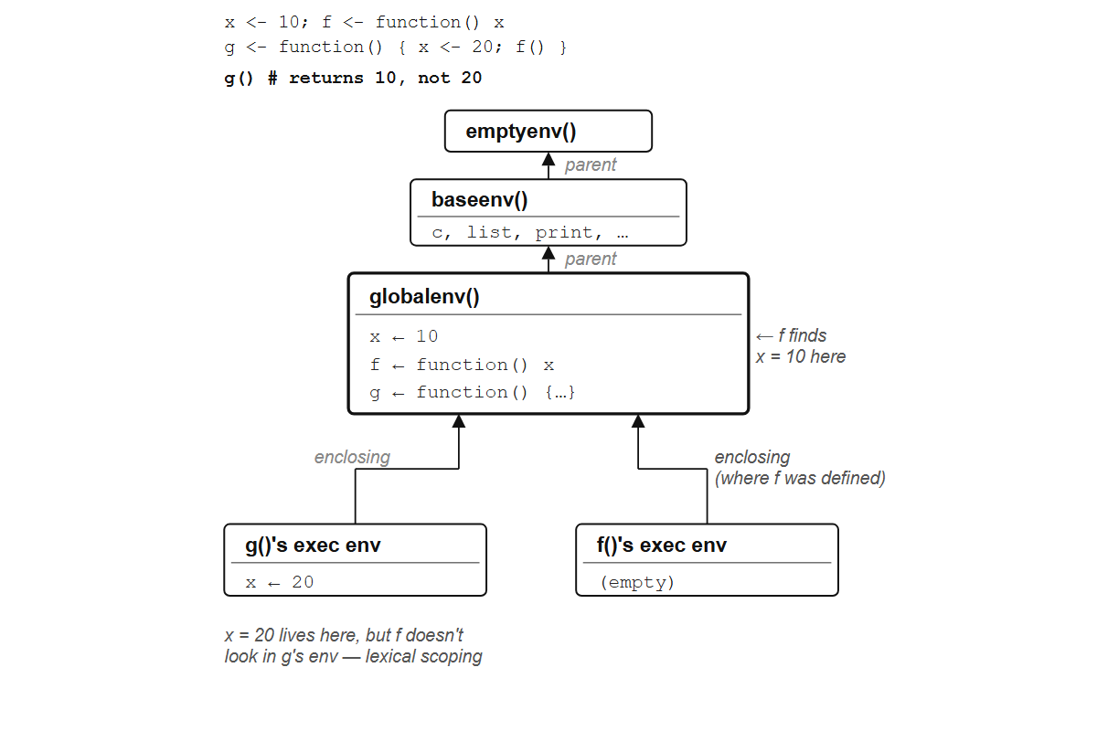
f finds x = 10 in the global environment where it was defined, not x = 20 in g’s execution environment.
You can inspect the current environment with environment(), list its contents with ls(), and find its parent with parent.env():
x <- 42
y <- "hello"
ls()
#> [1] "f" "x" "y"environment()
#> <environment: R_GlobalEnv>Functions remember things by holding a reference to the environment where they were created, which is why scope matters here.
18.1.1 The global environment
The global environment (.GlobalEnv, or equivalently globalenv()) is where your interactive work lives. Every time you type x <- 42 at the console, you create a binding here, at the bottom of the search path. It is also the default enclosing environment for any function you define interactively, and that default status has consequences.
identical(environment(), globalenv())
#> [1] TRUE
Three properties make it special. It never gets garbage-collected; it persists for the entire R session. Its parent is not fixed: it shifts whenever you attach a new package with library(). And it is the only environment you routinely modify by hand, because functions create and destroy their own execution environments automatically (Section 18.3), while the global environment simply accumulates bindings as you work.
That accumulation lets you explore interactively, building data objects step by step. It also means any function defined in the global environment can see and silently depend on those objects. A function that works in your current session may break in a fresh one because it relied on a global variable you forgot to pass as an argument.
In lambda calculus, that function is an open term: its result depends on bindings outside its own body. Pass all dependencies as arguments and it becomes a closed term, portable and self-contained. But what happens when a name isn’t passed as an argument?
18.1.2 The search path
When you type x at the console, R checks the global environment first; if no match turns up, it moves to the parent, then the parent’s parent, walking up the chain until it either finds the name or runs out of environments. This chain is the search path:
search()
#> [1] ".GlobalEnv"        "package:stats"     "package:graphics"
#> [4] "package:grDevices" "package:utils"     "package:datasets"
#> [7] "package:methods"   "Autoloads"         "package:base"
The global environment sits at the bottom, attached packages stack above it, and package:base lives near the top. That is why you can call mean() without writing base::mean(): R walks the chain, finds mean in the base package, and uses it. But the search path only governs lookups that start from the global environment. What governs lookups inside a function?
Exercises
- Run
ls()in a fresh R session. What do you see? Now assigna <- 1and runls()again. - Run
search()and count how many environments are in the chain. Load a package withlibrary(tools)and runsearch()again. Where did the new package appear? - What does
parent.env(globalenv())return? What aboutparent.env(baseenv())?
18.2 Lexical scoping
Consider this:
x <- 10
f <- function() x
g <- function() { x <- 20; f() }
g()
#> [1] 10
The result is 10, not 20. f was defined in the global environment, so it looks for x there, ignoring the x <- 20 inside g where it was merely called. This is lexical scoping: a function resolves names where it was defined, not where it was called.
The alternative, dynamic scoping, searches the call stack instead; the same function would return different results depending on who calls it. R got lexical scoping from Scheme (1975), not from S, which originally used dynamic scoping (Section 2.3); without it, closures would not work.
Four rules govern how R resolves names:
Name masking. Local names shadow names in parent environments. If a function defines
x, thatxhides anyxin the global environment.Functions vs variables. R distinguishes function lookups from variable lookups. If you call
f(3), R searches forfbut skips non-function values. This means you can have a variablec <- 10and still callc(1, 2, 3)to create a vector, because R knows you want the function.Fresh start. Every function call gets a fresh execution environment. Variables from a previous call don’t carry over.
Dynamic lookup. R looks up names when the function runs, not when it’s defined. If a function uses a free variable, its value can change between calls:
multiplier <- 2
scale <- function(x) x * multiplier
scale(5)
#> [1] 10
multiplier <- 10
scale(5)
#> [1] 50scale never snapshots the value of multiplier at definition time; it reaches into the enclosing environment fresh on every call, which means the function adapts automatically if multiplier changes. Occasionally useful. More often, a source of bugs: someone modifies a global variable, and a seemingly unrelated function starts returning different results, with nothing at the call site to explain why.
Exercises
Predict the output before running:
x <- 1
f <- function() {
  x <- 2
  g <- function() x
  g()
}
f()
Predict the output:
x <- 1
f <- function() {
  g <- function() x
  x <- 2
  g()
}
f()
Why is the result different from what you might expect? (Hint: rule 4.)
Can you have a variable named
meanand still call the functionmean()? Try it.
18.3 Execution environments
Every time you call a function, R creates a new environment (the execution environment) with the function’s arguments and local variables as bindings. That is why the counter at the top of this chapter never advances:
f <- function() {
  n <- 0
  n <- n + 1
  n
}

f()
#> [1] 1
f()
#> [1] 1
f()
#> [1] 1
Call it ten times, a hundred times; you always get 1, because each call gets its own execution environment with its own n, and the previous call’s n vanishes the moment that call returns (rule 3).
The parent of this fresh execution environment is not the environment where the function was called; it is the environment where the function was defined (the enclosing environment). This is what makes scoping lexical: the parent chain is determined by the structure of the source code, not by which function happened to call which at runtime.
x <- "global"

outer <- function() {
  x <- "outer"
  inner <- function() x
  inner()
}

outer()
#> [1] "outer"
inner was defined inside outer, so its enclosing environment is outer’s execution environment, and when inner looks for x, it finds "outer", not "global". But outer’s execution environment is temporary. Normally, local variables live and die with the call: when the function returns, its execution environment gets garbage-collected and everything inside it disappears.
Unless something keeps it alive. What if outer returned inner instead of calling it? What if a function escaped the environment where it was born, carrying a reference that prevented the garbage collector from reclaiming it?
Exercises
Write a function
fresh()that creates a local variablen <- 0, increments it, and returns it. Call it three times and verify you always get 1.Predict the output:
make <- function() {
  a <- 1
  function() a
}
h <- make()
a <- 99
h()
18.4 Closures
All R functions are technically closures (they all carry an enclosing environment), but the term earns its keep when a function captures variables from a parent that isn’t the global environment. Here is a counter that actually counts:
make_counter <- function() {
  n <- 0
  function() {
    n <<- n + 1
    n
  }
}

count <- make_counter()
count()
#> [1] 1
count()
#> [1] 2
count()
#> [1] 3
When you call make_counter(), R creates an execution environment with n <- 0. The inner function is defined in that environment, making it the inner function’s enclosing environment. When make_counter returns this inner function, the execution environment would normally be garbage-collected. The returned function still points to it, though, so it survives. Each subsequent call to count() creates its own fresh execution environment for its local work, but the enclosing environment (the one from make_counter that holds n) is shared across all calls, persistent as long as count exists. That is how count remembers its state between invocations.
But notice the <<-. That choice is not cosmetic.
<<- is the super-assignment operator. Instead of creating a local binding, it searches parent environments for an existing binding named n and modifies it in place. Without <<-, writing n <- n + 1 would create a local n in the execution environment, shadowing the captured one, and the counter would always return 1 (the same broken non-counter from the top of the chapter).
Two counters are independent, because each call to make_counter() creates a separate execution environment with its own n:
a <- make_counter()
b <- make_counter()
a()
#> [1] 1
a()
#> [1] 2
a()
#> [1] 3
b()
#> [1] 1
a has counted to 3; b has counted to 1. They share no state; each factory call minted a private universe. But the mechanism that keeps these universes alive is the same one that can leak state into the global environment if <<- is used carelessly.
Connection to Section 7.4: make_adder was a preview. Now you understand why the returned function remembers n: an environment stays alive because something still points to it.
In lambda calculus, the same thing happens through substitution. In make_adder(5), the returned function \(x) x + n has n as a free variable: a name that is used but not defined inside the function. The closure captures n = 5, binding that free variable. In lambda notation, make_adder is (λn. λx. x + n), and applying it to 5 gives λx. x + 5 by substitution (beta reduction), replacing the free variable n with a concrete value. Closures are the runtime mechanism that makes this substitution real. The name itself comes from this idea: a closure closes over its free variables, turning an open term (one with unresolved names) into a closed one (where every variable is accounted for).
Every closure you create in R is a beta reduction frozen mid-step. make_adder(5) reduces (λn. λx. x + n) to λx. x + 5, but the returned function doesn’t evaluate further until you give it an x. The closure holds the partially reduced term, waiting. When you finally call add5(3), another beta reduction fires: (λx. x + 5)(3) becomes 3 + 5, and R evaluates it to 8. Two reductions, two calls, one answer.
R does exactly this internally when it resolves the captured binding n = 5 in the enclosing environment. But <<- gave the closure something lambda calculus never had to worry about: the ability to mutate its captured bindings. That power needs guardrails.
Exercises
- Create a counter with
make_counter. Call it five times. Then inspect the capturednwithenvironment(count)$n. - Modify
make_counterto accept a starting value:make_counter <- function(start = 0) { ... }. Verify thatmake_counter(10)starts counting from 11. - Write
make_countdown(n)that counts down fromn. Each call returns the next value. What happens when it reaches 0?
18.5 <<- and mutable state
<<- is the only way to create mutable state in R’s functional world, because it searches parent environments for an existing binding and modifies it there. If it doesn’t find the variable in any parent, it creates one in the global environment. That is almost always a mistake.
rm(oops, envir = globalenv())  # clean slate
#> Warning in rm(oops, envir = globalenv()): object 'oops' not found
f <- function() {
  oops <<- "surprise"
}
f()
oops
#> [1] "surprise"
oops was never defined anywhere, so <<- walked all the way up the parent chain, found nothing, and quietly created it in the global environment. A side effect invisible at the call site, exactly the kind of hidden dependency that makes code hard to debug.
TipOpinion
Use <<- inside closures, never in top-level scripts. If you find yourself using <<- to modify a global variable, you are writing a bug you haven’t found yet. The legitimate use case is closures that encapsulate state: counters, caches, accumulators, where the modified variable lives in a private environment invisible to the outside world.
Inside a closure, <<- is safe precisely because the variable it modifies lives in the closure’s private environment, not in the global environment. Nobody outside the closure can see it or change it (unless they deliberately reach into the environment with environment(f)$n, which is an explicit, conscious choice, not an accident).
But safe is not the same as free. When you use <<-, the function gains memory — each call can depend on every previous call — and every reader of that function must now track two things: what happens inside the function body, and what state the enclosing environment carries from prior calls. Lambda calculus never had this problem because substitution is the only operation: (λn. λx. x + n)(5) reduces to λx. x + 5, and the 5 is baked in permanently, not stored in a mutable cell that some future call might overwrite. R’s closures give you the substitution and the mutable cell. That combination is what makes the counter work — each call to count() modifies n in the enclosing environment, and the next call sees the updated value. It is also what makes <<- bugs invisible from the call site: the one-character slip from n <<- n + 1 to n <- n + 1 produces no error and no warning, just a counter stuck at 1.
rm(oops, envir = globalenv())Exercises
- Write a closure
make_accumulator(start)that returns a function. Each call adds its argument to a running total and returns the new total. Test:acc <- make_accumulator(0); acc(5); acc(3); acc(10)should return 5, 8, 18. - What happens if you use
<-instead of<<-inside the closure? Try it with the counter example.
18.6 Closures as portable state
A closure bundles a function with its data: no global variables, no side effects visible from outside. Consider a function that must remember every value it has ever seen, a running mean that updates with each new observation:
make_running_mean <- function() {
  total <- 0
  count <- 0
  function(x) {
    total <<- total + x
    count <<- count + 1
    total / count
  }
}

avg <- make_running_mean()
avg(10)
#> [1] 10
avg(20)
#> [1] 15
avg(6)
#> [1] 12
A factory function creates an environment, returns an inner function that captures it, and <<- lets the inner function modify the captured state. The state lives in a private environment that travels with the function: no outside code can see or tamper with it, and it persists across calls.
The global-variable approach does none of this:
# Don't do this
total <- 0
count <- 0

running_mean <- function(x) {
  total <<- total + x
  count <<- count + 1
  total / count
}
This version pollutes the global environment with total and count, which any other code can read or modify; you cannot have two independent running means; and if you forget to reset them, your next analysis starts with stale state. The closure version has none of these problems, and its uses reach well beyond counters and accumulators:
- Function factories (Chapter 20): parameterized families of functions.
make_adder,make_multiplier, and their real-world cousins in ggplot2 themes, statistical tests, and data transformations. - Memoization: cache expensive results so they’re computed only once.
- Callbacks and event handlers: carry context without globals, common in Shiny applications.
- Encapsulated modules: a list of closures sharing a private environment.
That last pattern deserves a concrete example, because a list of closures sharing an environment is functionally equivalent to an object with methods and private fields:
make_bank_account <- function(balance = 0) {
  list(
    deposit  = function(amount) {
      balance <<- balance + amount
      invisible(balance)
    },
    withdraw = function(amount) {
      balance <<- balance - amount
      invisible(balance)
    },
    check    = function() balance
  )
}

acct <- make_bank_account(100)
acct$deposit(50)
acct$withdraw(30)
acct$check()
#> [1] 120
Three closures share a single environment containing one private variable, balance. From the outside, acct behaves like an object with methods; from the inside, it is just functions closing over a shared environment. Peter Norvig observed that “closures are poor man’s objects, and objects are poor man’s closures.” R6 works this way internally: each R6 object is an environment, and its methods are functions whose enclosing environment is that same environment. Chapter 24 explores where that equivalence leads.
Exercises
- Build a
make_running_meanclosure. Feed it the values 4, 8, 12. Verify the running mean is 4, 6, 8. - Create two independent running means,
avg1andavg2. Feed different values to each and verify they don’t interfere. - Extend
make_bank_accountwith astatementfunction that returns a character vector of all transactions (deposit or withdrawal). You’ll need ahistoryvariable in the enclosing environment.
18.7 Inspecting environments
Closures are easier to understand when you can look inside them. environment(f) returns the enclosing environment of a function, ls() lists what’s in it, and you can access captured variables directly with $:
count <- make_counter()
count()
#> [1] 1
count()
#> [1] 2

environment(count)
#> <environment: 0x000001ec9468d1c0>
ls(environment(count))
#> [1] "n"
environment(count)$n
#> [1] 2
The counter has been called twice, so n is 2. Watch it change:
count()
#> [1] 3
environment(count)$n
#> [1] 3
Now n is 3, incremented by the call.
For a richer view, rlang::env_print() shows the environment’s contents, parent, and memory address:
rlang::env_print(environment(count))These tools are not for production code (reaching into a closure’s environment breaks its encapsulation), but for learning they are the fastest way to see what a closure actually holds. Make one, inspect its environment, call it, inspect again. A closure that holds state and a list of closures that share an environment start to look a lot like an object with methods, which is exactly the connection Section 24.2 explores.
Exercises
- Create a running mean with
make_running_mean. Feed it three values. Then inspectenvironment(avg)$totalandenvironment(avg)$countto verify the internal state. - Create two counters. Inspect their environments and confirm they have different
nvalues after calling them different numbers of times. - What does
environment(mean)return? Why is it different fromenvironment(count)?