pop_wide <- data.frame(
  country    = c("Norway", "Sweden", "Denmark"),
  pop_2020   = c(5380, 10350, 5831),
  pop_2021   = c(5391, 10380, 5840),
  pop_2022   = c(5408, 10420, 5857)
)
pop_wide
#>   country pop_2020 pop_2021 pop_2022
#> 1  Norway     5380     5391     5408
#> 2  Sweden    10350    10380    10420
#> 3 Denmark 5831 5840 585716 Tidy data
You have a data frame with population figures for three countries, and the years are column names: pop_2020, pop_2021, pop_2022. You want to plot population over time, so you try mapping year to the x-axis. There is no year column. The information is there, hiding in plain sight, encoded in the syntax of your column headers rather than the semantics of your data. Every dplyr verb you learned in Chapter 14, every ggplot2 aesthetic you’ll ever write, every model formula you’ll ever fit: they all assume that each variable lives in its own column. When it doesn’t, nothing works. Getting data into the right shape occupies more of a working analyst’s time than any model or visualization, and yet most introductions to R treat it as an afterthought, something you do before the real work begins. This chapter treats it as the real work, because it is.
You already have the pieces: data frames from Chapter 11, verbs from Chapter 14, pipes from Chapter 15. What you’re missing is the target shape those tools expect.
16.1 What tidy means
Hadley Wickham’s 2014 paper “Tidy data” defines three rules:
- Each variable is a column.
- Each observation is a row.
- Each type of observational unit is a table.
They sound obvious. They aren’t. Most real-world data breaks at least one of them, and recognizing which rule is broken (let alone fixing it) takes practice.
Consider a table of population data with years spread across the column names:
What is the variable here? Year. But “year” doesn’t appear as a column; it’s buried inside the names pop_2020, pop_2021, pop_2022, three columns where there should be one. Not tidy.
These rules are a simplified version of something database designers have known since the 1970s, when Edgar Codd defined a set of normal forms to eliminate redundancy. The structural problem R programmers wrestle with today is the same one Codd solved in relational algebra before R existed.
The tidy version has three columns: country, year, and population. One variable per column, one observation per row, nine values arranged so that every tool you’ve learned can reach them.
pop_tidy <- data.frame(
  country    = rep(c("Norway", "Sweden", "Denmark"), each = 3),
  year       = rep(2020:2022, times = 3),
  population = c(5380, 5391, 5408, 10350, 10380, 10420, 5831, 5840, 5857)
)
pop_tidy
#>   country year population
#> 1  Norway 2020       5380
#> 2  Norway 2021       5391
#> 3  Norway 2022       5408
#> 4  Sweden 2020      10350
#> 5  Sweden 2021      10380
#> 6  Sweden 2022      10420
#> 7 Denmark 2020       5831
#> 8 Denmark 2021       5840
#> 9 Denmark 2022       5857
Now you can filter by year, group by country, plot year on the x-axis. Every dplyr verb and every ggplot2 aesthetic mapping works because each variable occupies its own column, and the tools compose because the data has a consistent shape. But who wants to rearrange nine values by hand?
Exercises
- Look at this table. Which tidy-data rule does it break?
data.frame(
  student = c("Alice", "Bob"),
  math_score = c(90, 85),
  english_score = c(78, 92)
)
Sketch (on paper or in a comment) what the tidy version of that table would look like. How many rows? How many columns?
A data frame has columns
name,date, andtemperature. One row per city per day. Is this tidy? Why or why not?
16.2 pivot_longer(): columns to rows
pivot_longer() from the tidyr package does the reshaping in one call:
library(tidyr)
library(dplyr)
#>
#> Attaching package: 'dplyr'
#> The following objects are masked from 'package:stats':
#>
#> filter, lag
#> The following objects are masked from 'package:base':
#>
#> intersect, setdiff, setequal, union
pop_wide |>
pivot_longer(
cols = pop_2020:pop_2022,
names_to = "year",
values_to = "population"
)
#> # A tibble: 9 × 3
#> country year population
#> <chr> <chr> <dbl>
#> 1 Norway pop_2020 5380
#> 2 Norway pop_2021 5391
#> 3 Norway pop_2022 5408
#> 4 Sweden pop_2020 10350
#> 5 Sweden pop_2021 10380
#> 6 Sweden pop_2022 10420
#> 7 Denmark pop_2020 5831
#> 8 Denmark pop_2021 5840
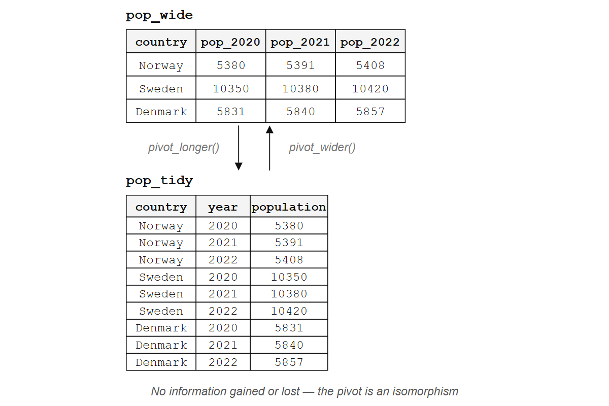
#> 9 Denmark pop_2022 5857Three countries, three years, nine population values: the information content is identical in both forms. pivot_longer() and pivot_wider() are inverses; applying one and then the other returns you to where you started (up to column ordering). A pair of reversible transformations like this is called an isomorphism: two structures that contain the same information in different arrangements. Wide and long formats are isomorphic; neither is “more correct.”
What changes when you pivot is the alignment between the data’s shape and your next tool’s expectations. A report reader wants wide, because scanning countries across years in a single row is easier than scrolling. A ggplot() call wants long, because each aesthetic maps to one column and each observation occupies one row. Grouped summaries need the grouping variable to be a column, not a set of column names baked into the header. Choosing a format is choosing which tool you are about to hand the data to, and pivoting is the translation between those expectations.
The hard part is not the reshaping itself but deciding what to reshape. Given an arbitrary table with merged cells, hierarchical headers, and embedded metadata, determining the correct tidy structure requires human judgment about what constitutes a variable, an observation, and a value. Wickham’s 2014 paper defines these three terms precisely to make that judgment tractable: once you answer “is year a variable or a value?”, the reshaping follows mechanically.
Three arguments control the transformation:
cols: which columns to pivot. Accepts tidy selection helpers likestarts_with(),where(is.numeric), or a range with:.names_to: what to call the new column made from column names.values_to: what to call the new column made from cell values.
The column names still carry the pop_ prefix, and year is character, not integer. Two more arguments fix that:
pop_wide |>
  pivot_longer(
    cols            = pop_2020:pop_2022,
    names_to        = "year",
    names_prefix    = "pop_",
    names_transform = list(year = as.integer),
    values_to       = "population"
  )
#> # A tibble: 9 × 3
#>   country  year population
#>   <chr>   <int>      <dbl>
#> 1 Norway   2020       5380
#> 2 Norway   2021       5391
#> 3 Norway   2022       5408
#> 4 Sweden   2020      10350
#> 5 Sweden   2021      10380
#> 6 Sweden   2022      10420
#> 7 Denmark  2020       5831
#> 8 Denmark  2021       5840
#> 9 Denmark  2022       5857
names_prefix strips the leading text; names_transform applies a function to the extracted names, here converting character years to integers.
For more complex column names, names_sep and names_pattern let you split structured names into multiple new columns. If you had columns like bill_length_mm and bill_depth_mm, you could split on _ to extract both the measurement and the unit. The tidyr pivoting vignette covers these cases in detail. But what about the opposite direction, when your data is too long?
Exercises
- Create this data frame and pivot it to tidy form with columns
city,quarter, andsales:
quarterly <- data.frame(
  city = c("Oslo", "Bergen"),
  Q1   = c(120, 95),
  Q2   = c(135, 110),
  Q3   = c(150, 105),
  Q4   = c(160, 130)
)
Modify your pivot to strip the
Qprefix from the quarter column and convert it to an integer.What happens if you set
values_toto the name of an existing column? Try it.
16.3 pivot_wider(): rows to columns
Sometimes the problem goes the other way: distinct variables are stacked into a single column, and you need to spread them out.
measurements <- data.frame(
  site        = rep(c("A", "B"), each = 2),
  measurement = rep(c("temperature", "humidity"), times = 2),
  value       = c(22.1, 65, 19.8, 72)
)
measurements
#>   site measurement value
#> 1    A temperature  22.1
#> 2    A    humidity  65.0
#> 3    B temperature  19.8
#> 4    B    humidity  72.0
Temperature and humidity are different variables, and cramming them into a single value column conflates two things that should be separate. pivot_wider() pulls them apart:
measurements |>
  pivot_wider(
    names_from  = measurement,
    values_from = value
  )
#> # A tibble: 2 × 3
#>   site  temperature humidity
#>   <chr>       <dbl>    <dbl>
#> 1 A            22.1       65
#> 2 B            19.8       72
Two arguments:
names_from: which column’s values become the new column names.values_from: which column’s values fill the new cells.
When some combinations don’t exist in the data, pivot_wider() fills those cells with NA. The values_fill argument lets you choose a different default:
incomplete <- data.frame(
  site        = c("A", "A", "B"),
  measurement = c("temperature", "humidity", "temperature"),
  value       = c(22.1, 65, 19.8)
)

incomplete |>
  pivot_wider(
    names_from  = measurement,
    values_from = value,
    values_fill = 0
  )
#> # A tibble: 2 × 3
#>   site  temperature humidity
#>   <chr>       <dbl>    <dbl>
#> 1 A            22.1       65
#> 2 B            19.8        0
TipOpinion
If you reach for pivot_wider() during analysis, pause and ask whether your downstream tool really needs wide data. Usually it doesn’t. pivot_wider() is most useful for building display tables and for feeding data into functions that expect matrix-like input. The fact that wide format looks tidier to human eyes doesn’t mean it is tidier for your code.
Exercises
Start with
pop_tidy(the tidy population table from Section 16.1). Usepivot_wider()to recreate the wide format, with one column per year.What happens if the combination of id columns isn’t unique before widening? Create a data frame where two rows have the same
siteandmeasurementand trypivot_wider(). Read the warning.
16.4 When data isn’t tidy (and that’s fine)
Tidy data is for analysis. Not every use case is analysis.
Wide tables are easier for humans to scan: a table with countries as rows and years as columns fits on a screen, while the same data in long form might scroll for hundreds of rows. Wide format is also what some matrix operations, correlation computations, and model interfaces expect when they want one column per predictor.
Data entry follows the same logic. If you’re recording daily temperatures for three cities, a spreadsheet with cities as rows and dates as columns feels natural; nobody fills in a three-column long-form table by hand (and anyone who tells you they do is lying, or masochistic, or both).
So reshape to tidy when you need dplyr and ggplot, reshape to wide when you need a human to read the table. Do not get religious about it.
Sometimes the information you need spans multiple tables.
16.5 Joins: combining tables
You have customers and orders, species and observations, sites and measurements. The data lives in separate tables, linked by a shared key. Joins are how you bring them together.
bands <- data.frame(
  name  = c("John", "Paul", "George", "Ringo"),
  plays = c("guitar", "bass", "guitar", "drums")
)

albums <- data.frame(
  name  = c("John", "Paul", "George", "Mick"),
  album = c("Imagine", "Ram", "All Things Must Pass", "Some Girls")
)
Mutating joins
Mutating joins add columns from the second table to the first.
left_join() keeps all rows from the left table and attaches matching columns from the right, filling NA where no match exists:
bands |> left_join(albums, by = "name")
#>     name  plays                album
#> 1   John guitar              Imagine
#> 2   Paul   bass                  Ram
#> 3 George guitar All Things Must Pass
#> 4  Ringo  drums                 <NA>
Ringo has no album in the albums table, so his album comes back NA; Mick has no row in bands, so he’s dropped entirely. This is the workhorse join: keep everything on the left, enrich with what you can from the right.
inner_join() is stricter, keeping only rows that match in both tables:
bands |> inner_join(albums, by = "name")
#>     name  plays                album
#> 1   John guitar              Imagine
#> 2   Paul   bass                  Ram
#> 3 George guitar All Things Must Pass
Ringo and Mick are both gone. Only the three names appearing in both tables survive.
When the key columns have different names, use join_by():
instruments <- data.frame(
  musician   = c("John", "Paul", "George", "Ringo"),
  instrument = c("guitar", "bass", "guitar", "drums")
)

albums |> left_join(instruments, by = join_by(name == musician))
#>     name                album instrument
#> 1   John              Imagine     guitar
#> 2   Paul                  Ram       bass
#> 3 George All Things Must Pass     guitar
#> 4   Mick           Some Girls       <NA>
Filtering joins
Filtering joins don’t add columns. They filter rows.
semi_join() keeps rows in the left table that have a match in the right:
bands |> semi_join(albums, by = "name")
#>     name  plays
#> 1   John guitar
#> 2   Paul   bass
#> 3 George guitar
Same three rows as inner_join(), but without the album column. You’re using albums as a filter, not as a source of new data.
anti_join() does the opposite, keeping rows in the left table that have no match in the right:
bands |> anti_join(albums, by = "name")
#>    name plays
#> 1 Ringo drums
Only Ringo: the one band member with no album in the albums table. anti_join() is your best tool for finding what’s missing. Which customers placed no orders? Which species have no observations? Which students didn’t submit?
TipOpinion
Start with left_join(). Use anti_join() to debug. The others are situational. right_join() exists but is rarely needed: swap the table order and use left_join() instead. full_join() keeps everything from both sides, which sounds safe but usually signals that you haven’t decided what your unit of analysis actually is.
Exercises
Create two small data frames:
studentswith columnsidandname, andgradeswith columnsidandscore. Give them overlapping but not identicalidvalues. Useleft_join()to combine them.Use
anti_join()on the same tables to find students with no grades and grades with no student. (Hint: swap which table is on the left.)What is the difference between
semi_join(bands, albums, by = "name")andinner_join(bands, albums, by = "name") |> select(name, plays)? Try both.
16.6 Other tidyr tools
Pivoting handles structure; joins handle combination. A handful of other tidyr functions handle the messy details that remain after those two big moves.
Separating and uniting columns
separate_wider_delim() splits one column into several by a delimiter:
dates <- data.frame(
  id   = 1:3,
  date = c("2024-03-15", "2024-07-22", "2024-11-01")
)

dates |>
  separate_wider_delim(
    cols  = date,
    delim = "-",
    names = c("year", "month", "day")
  )
#> # A tibble: 3 × 4
#>      id year  month day
#>   <int> <chr> <chr> <chr>
#> 1     1 2024  03    15
#> 2     2 2024  07    22
#> 3     3 2024  11    01
This replaces the older separate(), which relied on position-based splitting and was less predictable. For complex patterns, separate_wider_regex() lets you use regular expressions.
unite() does the inverse, pasting columns together:
data.frame(year = 2024, month = "03", day = 15) |>
  unite(col = "date", year, month, day, sep = "-")
#>         date
#> 1 2024-03-15
Completing and filling
complete() makes implicit missing values explicit. If your data has observations for some year/site combinations but not all, complete() adds rows for the gaps and fills them with NA:
obs <- data.frame(
  year = c(2020, 2020, 2021),
  site = c("A", "B", "A"),
  count = c(5, 3, 7)
)

obs |> complete(year, site)
#> # A tibble: 4 × 3
#>    year site  count
#>   <dbl> <chr> <dbl>
#> 1  2020 A         5
#> 2  2020 B         3
#> 3  2021 A         7
#> 4  2021 B        NA
fill() propagates the last non-missing value downward (or upward), which is useful for data where group labels are only written once and the rows beneath are left blank:
report <- data.frame(
  group = c("Control", NA, NA, "Treatment", NA),
  value = c(10, 12, 11, 20, 22)
)

report |> fill(group)
#>       group value
#> 1   Control    10
#> 2   Control    12
#> 3   Control    11
#> 4 Treatment    20
#> 5 Treatment    22
Nesting
nest() packs subsets of a data frame into list-columns, and unnest() unpacks them. This pattern shines when fitting models to groups, but it requires familiarity with list-columns and iteration, both covered in Section 19.3.
16.7 Summary
Tidy data is a structural contract: one variable per column, one observation per row, one observational unit per table. pivot_longer() turns columns into rows (the common direction), pivot_wider() turns rows into columns (the occasional direction), and joins combine tables by matching keys.
NoteThe mathematics underneath
These tools compose precisely because they all expect the same shape, and the connection to their mathematical foundations runs deeper than most R programmers realize. Codd’s relational algebra and the simply typed lambda calculus are both built on function application and composition over structured types, which is why the same ideas keep surfacing in R, SQL, and formal logic. In category theory, a join is a pullback: given two tables that each map to a shared key space, the join constructs the most general table consistent with both. Think of it as a Venn diagram for rows, where the overlap is determined by the key column; inner_join keeps only the overlap, while left_join keeps everything on the left and fills the gaps with NA.
But shape is only half the story. Once your data is tidy, you still need to do something with it, and doing the same thing to many groups, many columns, or many models at once is where iteration enters. That’s next.