28  Performance

So here is where you stand: you can find bottlenecks, eliminate unnecessary copies, hand tight loops to compiled code, and split independent work across cores. But the optimization that actually matters most is still the one at the top of the list. Measure first. Your profiler will catch things your intuition misses every time.

Your code is too slow. You know this because you ran it, waited, checked your phone, looked back at the screen, and it was still running. The question is: which part?

Most R code finishes before you notice it started. When something takes too long, the question is where the seconds go, and the answer is almost never where you expect. Profile first. After that, the fix depends on what the profiler shows: sometimes it is a vectorization you missed, sometimes a copy you did not know was happening, sometimes a loop that belongs in C++. The tools in this chapter cover all of those, and ?sec-connecting-to-other-languages covers the compiled-code path in detail.

28.1 Profile before you optimize

The function you suspect is slow is, more often than not, innocent. Some other line, one you barely glanced at while writing, runs a million times while the suspect runs once. Optimization without measurement is guesswork dressed up as engineering. You have to measure.

Quick timing with system.time():

system.time({
  x <- rnorm(1e6)
  y <- cumsum(x)
})
#>    user  system elapsed 
#>    0.03    0.00    0.02

The first number (user) is CPU time. The third (elapsed) is wall-clock time. Good enough for ballpark estimates, but ballpark estimates deceive you when differences are small, when the thing you are comparing takes three milliseconds and the noise takes five.

Precise benchmarking with bench::mark():

bench::mark(
  sqrt = sqrt(x),
  power = x^0.5,
  check = TRUE
)

bench::mark() runs each expression multiple times, reports median time and memory allocation, and checks that all expressions return the same result. Use it for head-to-head comparisons. microbenchmark::microbenchmark() is the older alternative: sub-millisecond accurate, runs expressions 100 times by default, reports summary statistics. Both work well; bench::mark is newer and checks for equal results automatically.

Profiling with profvis::profvis():

profvis::profvis({
  data <- read.csv("large_file.csv")
  cleaned <- dplyr::filter(data, !is.na(value))
  model <- lm(value ~ group, data = cleaned)
  summary(model)
})

profvis produces an interactive flame graph showing which lines eat the most time and allocate the most memory. Use it when you do not know where the bottleneck is, which, if you are honest with yourself, is most of the time.

Here is a concrete example. The function slow_analysis generates data, fits a model, copies residuals in a loop (using c() to grow a vector), and computes a summary:

slow_analysis <- function(n = 5e4) {
  x <- rnorm(n)
  y <- 2 * x + rnorm(n, sd = 0.5)
  df <- data.frame(x = x, y = y)
  fit <- lm(y ~ x, data = df)

  # The bottleneck: growing a vector one element at a time
  residuals_copy <- c()
  for (i in seq_len(n)) {
    residuals_copy <- c(residuals_copy, fit$residuals[i])
  }
  summary(fit)
}

profvis::profvis(slow_analysis(5e4))

The profile output shows where time actually goes:

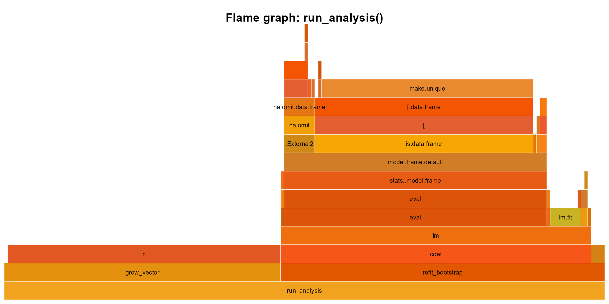
Figure 28.1: Flame graph of slow_analysis(): width is time. The c() tower on the left (the residual-copying loop) and the lm call stack on the right are the two hot spots. The c() loop takes roughly half the total time.

Read from bottom to top. slow_analysis calls lm on the right and runs the residual-copying loop on the left; inside the loop, nearly all time goes to c(), the vector-growing bottleneck, while inside lm the cost distributes across its internals (model.frame, eval, lm.fit). Without this graph, you might guess model fitting is the problem. The graph says otherwise.

The workflow is simple: run profvis on realistic input, find the hot spot, fix that one thing, re-profile. What do you do once you have found the bottleneck?

TipOpinion

If you have not profiled, you do not have a performance problem. You have a feeling.

Exercises

1. Use system.time() to compare sort(x) and x[order(x)] for x <- rnorm(1e6).
2. Use bench::mark() to compare sum(x) and Reduce("+", x) for x <- rnorm(1e4). Which is faster, and by how much?

28.2 Vectorization

Consider a vector of a million numbers. You want to double each one. You could write a loop that visits each element, multiplies it by two, stores the result. Or you could write x * 2 and let R handle the iteration. The second version runs 10 to 100 times faster. Why?

The answer traces back to 1962, when Kenneth Iverson at Harvard published A Notation as a Tool of Thought, describing APL (A Programming Language). APL’s central insight was that mathematical operations should apply to entire arrays, not individual elements: you do not write a loop to add two vectors; you write A + B and the language handles the rest. Iverson won the Turing Award for this work in 1979, and the idea traveled through S (where Chambers adopted it for statisticians who think in columns, not cells) and into R, where x * 2 multiplies every element of x without a loop, an index variable, or any mention of how many elements x contains.

When you call a vectorized function, R dispatches to optimized C code underneath. The loop still happens, but it happens in compiled machine code rather than stepping through R’s interpreter one element at a time. Think of it as the difference between reading a book aloud word by word and handing the entire manuscript to a speed-reader: the same work gets done, but the overhead per unit collapses.

x <- rnorm(1e5)

# Vectorized: fast
system.time(y <- x * 2)
#>    user  system elapsed 
#>       0       0       0

# Loop: slow
system.time({
  y <- numeric(length(x))
  for (i in seq_along(x)) y[i] <- x[i] * 2
})
#>    user  system elapsed 
#>       0       0       0

The difference grows with input size, and part of the speedup has nothing to do with R at all. Vectorized operations work on contiguous memory with sequential access patterns that the CPU prefetcher predicts correctly; sum(x) on a contiguous vector can be 100x faster than summing the same values scattered in a list, because L1 cache is roughly 27x faster than main memory. Martin Thompson, a high-performance computing advocate who borrowed the term from racing driver Jackie Stewart, calls this mechanical sympathy: writing software that works with the hardware rather than against it.

Common vectorization patterns:

Replace for + if with ifelse() or dplyr::case_when():

# Slow
result <- character(length(x))
for (i in seq_along(x)) {
  if (x[i] > 0) result[i] <- "pos" else result[i] <- "neg"
}

# Fast
result <- ifelse(x > 0, "pos", "neg")

Replace for + accumulate with cumsum(), cumprod(), cummax():

# Slow
result <- numeric(length(x))
result[1] <- x[1]
for (i in 2:length(x)) result[i] <- result[i-1] + x[i]

# Fast
result <- cumsum(x)

Replace loop-based row/column operations with rowSums(), colMeans(), matrix operations:

# Slow
row_totals <- numeric(nrow(mat))
for (i in 1:nrow(mat)) row_totals[i] <- sum(mat[i, ])

# Fast
row_totals <- rowSums(mat)

Not everything yields to vectorization. Iterations where each step depends on the previous result (Markov chains, recursive algorithms, some simulations) genuinely need loops, and for those Section 28.6 offers an escape hatch. But before reaching for compiled code, make sure you are not confusing convenience wrappers with the real thing.

sapply() and lapply() look like vectorization. They are not. They are convenient wrappers around loops that still call your R function once per element, no faster than a well-written for loop. True vectorization means the loop runs in C: sum(), cumsum(), ifelse(), pmin(), rowSums(). If the loop is still in R, the speed is still in R.

The distinction traces back to R’s inheritance. S was designed for interactive data analysis, not for writing loops. When John Chambers built S at Bell Labs, and when R’s creators reimplemented it at Auckland, the assumption was that heavy computation would happen in compiled Fortran or C routines, and the user-facing language would orchestrate those routines at a high level. Functions like sum() and rowSums() exist because they are the compiled routines, exposed directly. When you call sum(x), a single trip into C walks the memory block in a tight loop and returns the result. sapply(x, f) never leaves the interpreter; it calls your R function once per element, paying the full cost of argument matching, environment creation, and promise evaluation on every iteration. The speed gap between these two paths reflects a design choice that predates R itself: the language was built to orchestrate compiled routines, and code that stays in the interpreter is working against that architecture rather than with it.

So what happens when you have a loop that genuinely cannot be vectorized, but it still needs to be fast?

Exercises

1. Write a loop that computes the absolute value of each element in a vector. Then write the vectorized version using abs(). Benchmark both with bench::mark().
2. Replace this loop with a single vectorized expression: for (i in 1:length(x)) if (x[i] < 0) x[i] <- 0. (Hint: pmax().)

28.3 Memory: pre-allocate and avoid copies

A loop might be slow not because loops are inherently slow in R, but because R is copying your entire result vector on every iteration.

# Slow: O(n^2) because each c() copies the entire vector
slow_squares <- function(n) {
  result <- c()
  for (i in 1:n) result <- c(result, i^2)
  result
}

# Fast: O(n) with pre-allocation
fast_squares <- function(n) {
  result <- numeric(n)
  for (i in 1:n) result[i] <- i^2
  result
}

# Fastest: vectorized
vec_squares <- function(n) (1:n)^2

bench::mark(
  growing  = slow_squares(1000),
  prealloc = fast_squares(1000),
  vector   = vec_squares(1000),
  check = FALSE
)
#> # A tibble: 3 × 6
#>   expression      min   median `itr/sec` mem_alloc `gc/sec`
#>   <bch:expr> <bch:tm> <bch:tm>     <dbl> <bch:byt>    <dbl>
#> 1 growing     429.1µs  490.4µs     1918.    3.88MB   156.  
#> 2 prealloc     15.3µs   16.9µs    58190.   25.78KB     5.82
#> 3 vector          1µs    1.3µs   662496.   11.81KB   133.

Each call to c(result, value) allocates a new vector of size length(result) + 1 and copies every existing element into it. For n iterations, that totals \(1 + 2 + 3 + \cdots + n = O(n^2)\) copies, which means doubling your input size quadruples your runtime. Pre-allocation sidesteps the entire problem: you tell R the final size upfront with numeric(n), character(n), logical(n), or vector("list", n), and each assignment writes directly into the slot without copying anything.

But pre-allocation only solves the allocation problem. There is a second performance trap hiding in how R shares memory.

Copy-on-modify: R copies an object when you modify it and another name points to it:

x <- 1:1e6
y <- x        # y and x share the same memory
y[1] <- 0L    # now R copies, because modifying y would change x

You can track copies with tracemem():

x <- 1:5
tracemem(x)
#> [1] "<000001E803E115E8>"
y <- x
y[1] <- 0L    # triggers a copy
#> tracemem[0x000001e803e115e8 -> 0x000001e80dcc26e8]: eval eval withVisible withCallingHandlers eval eval with_handlers doWithOneRestart withOneRestart withRestartList doWithOneRestart withOneRestart withRestartList withRestarts <Anonymous> evaluate in_dir in_input_dir eng_r block_exec call_block process_group withCallingHandlers with_options <Anonymous> process_file <Anonymous> <Anonymous> execute .main
untracemem(x)

When only one name references an object, R modifies it in place, which is why pre-allocated loops are fast: the result vector has a single reference, so result[i] <- value writes directly without triggering a copy. The subtlety is that functions create references too. When you pass x to a function, the function parameter and the caller’s variable both point to the same object; if the function modifies its copy, R silently allocates a new one. This means helper functions called inside tight loops can trigger copies you never intended. tracemem() is your diagnostic tool here.

Exercises

1. Write a function that grows a character vector by appending one element at a time in a loop. Time it for n = 10000. Then rewrite with pre-allocation. What is the speedup?
2. Use tracemem() to observe when R copies a vector. Create x <- 1:5, then y <- x, then modify y[1] <- 99L. How many copies happen?

28.4 data.table

You have vectorized your operations, pre-allocated your loops, and the code is still too slow. The bottleneck is the data frame engine itself. dplyr is readable and expressive, but on millions of rows its abstractions carry a cost: intermediate copies, grouped operations that could be fused, filters that scan more data than necessary.

data.table strips away those abstractions:

library(data.table)

dt <- fread("large_file.csv")  # much faster than read.csv()

# Filter, compute, group in one expression
dt[age > 30, .(mean_income = mean(income)), by = region]

The dt[i, j, by] syntax puts row filtering (i), column operations (j), and grouping (by) in a single expression, which lets data.table optimize the entire operation as a single pass. It modifies columns in place (no copy-on-modify overhead), automatically parallelizes grouped operations, uses less memory than equivalent dplyr pipelines, and its fread() reads CSV files much faster than read.csv() and often faster than readr::read_csv().

The trade-off is a steeper learning curve; the dt[i, j, by] idiom reads differently from dplyr pipes. If you do not want to learn the syntax, dtplyr bridges the gap: write dplyr verbs, get data.table speed. It translates your pipeline behind the scenes.

A quick comparison:

# dplyr
library(dplyr)
sales |>
  filter(year == 2024) |>
  group_by(region) |>
  summarise(total = sum(revenue))

# data.table
library(data.table)
dt <- as.data.table(sales)
dt[year == 2024, .(total = sum(revenue)), by = region]

On small data, the difference is negligible. On millions of rows with many groups, the gap opens up:

n <- 5e6
sales <- data.frame(
  region = sample(letters, n, replace = TRUE),
  revenue = rnorm(n, 1000, 200)
)
dt <- data.table::as.data.table(sales)

bench::mark(
  dplyr = sales |>
    dplyr::group_by(region) |>
    dplyr::summarise(total = sum(revenue)),
  data.table = dt[, .(total = sum(revenue)), by = region],
  check = FALSE
)
# data.table is typically 3-10x faster on grouped aggregations at this scale.
# The gap widens with more groups and more rows.

Reach for data.table when your data has millions of rows, when you are grouping over many categories, or when the same pipeline runs repeatedly in a loop or a Shiny app. If your data fits comfortably in memory and dplyr finishes in seconds, switching buys you nothing but a syntax change. Both dplyr and data.table operate entirely in memory. data.table still loads the entire dataset into RAM before it touches a single row.

Exercises

1. Install data.table and convert mtcars to a data.table with as.data.table(). Compute the mean mpg grouped by cyl using the dt[i, j, by] syntax. Verify your result matches mtcars |> group_by(cyl) |> summarise(mean(mpg)).
2. Use fread() to read a CSV file (any file you have, or write one with fwrite(mtcars, "test.csv") first). Compare its speed against read.csv() using bench::mark().

28.5 Columnar engines: Arrow and DuckDB

What happens when your data no longer fits in memory, or when it does fit but you want analytics that finish before your coffee cools?

You have probably already hit the wall. A grouped summarise() on 50 million rows takes minutes and turns your laptop fan into a jet engine. read.csv() on a 10 GB file eats all available RAM and crashes the session without producing a single result. The data is not even big by industry standards; R just was not designed to hold it all at once and churn through it.

Arrow (arrow package) reads Parquet and Feather files and processes them with dplyr syntax. Operations are lazy: they build a query plan, then execute it in a single pass, loading only the columns and rows you actually need:

library(arrow)

open_dataset("data/large_parquet/") |>
  dplyr::filter(year == 2024) |>
  dplyr::group_by(region) |>
  dplyr::summarise(total = sum(revenue)) |>
  dplyr::collect()  # only now does data enter R

DuckDB (duckdb package) is an embedded analytical database that reads Parquet, CSV, and data frames, handles data larger than RAM, and supports both SQL and dplyr syntax (via dbplyr):

library(duckdb)
con <- dbConnect(duckdb())
duckdb_register(con, "sales", sales_df)

dbGetQuery(con, "SELECT region, SUM(revenue) FROM sales GROUP BY region")
dbDisconnect(con)

duckplyr removes the SQL entirely: it is a drop-in replacement for dplyr that routes computation through DuckDB’s engine. Same syntax, faster execution, near-zero transition cost. In June 2025, duckplyr formally joined the tidyverse. Existing dplyr code runs unchanged; duckplyr intercepts the verbs, routes what it can through DuckDB, and falls back to dplyr for anything DuckDB does not support.

The stack looks like this: Parquet files on disk, Arrow or DuckDB as the engine, dplyr verbs as the interface, results collected into R. You write the same code you already know; the machinery underneath is faster. Much of that speed comes from query fusion, combining multiple operations into a single pass over the data and eliminating intermediate allocations. In functional programming, this technique is called deforestation (Wadler, 1988): map f . map g creates an intermediate list, but fusion rewrites it as map (f . g), traversing the data once. data.table and Arrow apply the same principle at scale.

The dplyr verbs from Chapter 14 were designed as a functional interface: data frame in, data frame out, no mutation of the input. data.table, Arrow, DuckDB, and Polars are all different engines, written in different languages (C, C++, Rust), with different memory layouts and different optimization strategies. The dplyr verbs sit on top of all of them unchanged. filter(), mutate(), summarise() work on a local data frame, on a Parquet file through Arrow, on a DuckDB table through duckplyr. Four engines have appeared since dplyr was designed, and the interface has not changed once.

TipOpinion

If your data fits in memory and dplyr is fast enough, stop. If it does not fit, or if grouped aggregations drag, try DuckDB. With duckplyr the transition cost is nearly zero.

Exercises

1. Install duckdb and DBI. Create an in-memory DuckDB connection, register mtcars as a table, and run a SQL query to compute mean mpg grouped by cyl. Compare the result with your data.table answer from the previous section.
2. If you have a Parquet file (or create one with arrow::write_parquet(mtcars, "test.parquet")), open it with arrow::open_dataset(), filter, and collect(). Verify the result matches the equivalent dplyr operation on the in-memory data frame.

28.6 When and how to call compiled code

Sometimes R is simply the wrong language for the inner loop. You have profiled, vectorized, pre-allocated, tried data.table, and the bottleneck is a tight loop where each iteration depends on the last, where no vectorized function exists, where the work is purely computational and measured in millions of iterations. At that point, the right move is to write the hot loop in a compiled language and call it from R. Three options: C, C++ (via Rcpp), and Rust (via extendr).

C via .Call(): R’s native foreign function interface. You write C functions that take and return SEXP objects (R’s internal type), managing memory yourself with PROTECT/UNPROTECT:

// sum_c.c
#include <R.h>
#include <Rinternals.h>

SEXP sum_c(SEXP x) {
    double total = 0;
    for (int i = 0; i < length(x); i++) {
        total += REAL(x)[i];
    }
    return ScalarReal(total);
}

Low-level, no dependencies, maximum control. Used extensively in base R and older packages.

C++ via Rcpp: the most popular choice, and for good reason. It handles type conversion and memory management automatically, so you write code that looks almost like normal C++:

// sum_cpp.cpp
#include <Rcpp.h>
using namespace Rcpp;

// [[Rcpp::export]]
double sum_cpp(NumericVector x) {
    double total = 0;
    for (int i = 0; i < x.size(); i++) {
        total += x[i];
    }
    return total;
}

Rcpp::sourceCpp("sum_cpp.cpp") compiles and loads the function in one step. Immediate gratification.

Rust via extendr: the newest option. Rust provides memory safety without garbage collection; segfaults are, by design, impossible in safe Rust:

// sum_rust.rs
use extendr_api::prelude::*;

#[extendr]
fn sum_rust(x: &[f64]) -> f64 {
    x.iter().sum()
}

rextendr::rust_function() for interactive use, rextendr::use_extendr() to set up a Rust-powered package. The ecosystem is young but growing fast.

When to reach for compiled code:

• Loops where each iteration depends on the previous one.
• Recursive algorithms (tree traversal, dynamic programming).
• Operations that process each element individually (no vectorization possible).
• Hot loops identified by profiling.

When not to: when vectorization solves the problem, when the bottleneck is I/O (more C++ will not make your disk spin faster), when correctness matters more than speed and the compiled code would be complex enough to harbor bugs.

TipOpinion

The three options are not interchangeable items on a menu; they sit at different points on a genuine trade-off. Rcpp gives you the deepest ecosystem and the smoothest on-ramp, but nothing stops you from writing a buffer overrun that corrupts memory silently and crashes R ten minutes later. Rust catches those errors at compile time, before your code ever runs, but its R integration is younger and the community smaller, so you will find fewer examples and hit more rough edges. Raw C gives you total control and zero dependencies at the cost of managing every allocation yourself.

Start with Rcpp. It has the largest community, the most examples, and the gentlest on-ramp. Consider Rust if you want compile-time safety guarantees. Consider raw C only if you need zero dependencies.

28.7 The optimization checklist

When code is too slow, work through this list in order:

1. Profile: find the bottleneck. Do not guess.
2. Vectorize: replace element-wise loops with vectorized operations.
3. Pre-allocate: if you must loop, pre-allocate the result.
4. Algorithm: sometimes the problem is \(O(n^2)\) and the fix is \(O(n \log n)\). Better algorithms beat faster languages.
5. data.table or DuckDB: for large data, switch the engine.
6. Compiled code (Rcpp, extendr, .Call()): for tight loops that cannot be vectorized.
7. Parallelize: future.apply, furrr, parallel. Adds concurrency complexity; worth it when the bottleneck is embarrassingly parallel.

Profiling comes first because Amdahl’s law (1967) puts a hard ceiling on what any optimization can gain. If 5% of your code takes 95% of the time, making the other 95% infinitely fast yields only a 5% speedup. The same limit applies to parallelization: if 10% of the work is sequential, you can never exceed a 10x speedup no matter how many cores you throw at it. You need to know which 5% to fix before choosing how to fix it.

R offers several frameworks for parallel execution. parallel::mclapply() works on Unix but not Windows. future.apply::future_lapply() works everywhere and swaps in for lapply() with minimal changes. furrr::future_map() is the parallel version of purrr::map(). All split work across cores, and all carry the same caveat: parallelization only helps when the work is CPU-bound and divisible. If the bottleneck is reading from disk, more cores will not help. If iterations depend on each other, you cannot split them. And the overhead of spawning workers and collecting results means parallelization only pays off when each unit of work is substantial (milliseconds, not microseconds).

library(future.apply)
plan(multisession, workers = 4)

# Parallel version of sapply
results <- future_sapply(1:100, function(i) {
  # some expensive computation
  Sys.sleep(0.1)
  i^2
})