add_tax <- function(price, rate) price * (1 + rate)

prices <- c(10, 25, 8, 42)
with_tax <- sapply(prices, add_tax, rate = 0.2)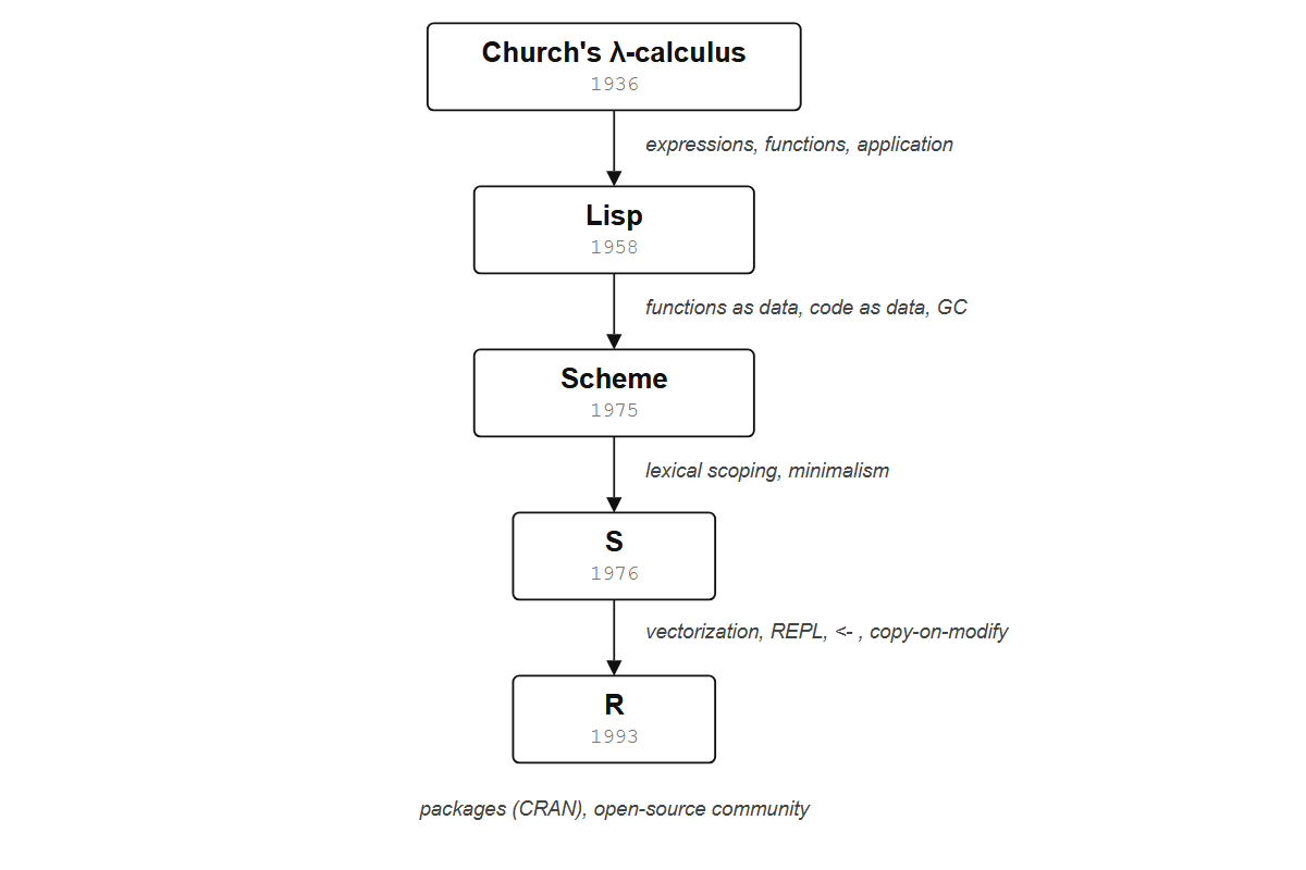
with_tax2 R’s family tree
Consider this small program in R:
That code used four ideas R did not invent: first-class functions, vectorized operations, higher-order functions, and lexical scope. They arrived from different languages and different decades.
2.1 Church’s lambda calculus becomes a programming language
By 1958, the only real option for writing programs was Fortran, which John Backus and his team at IBM had released the year before. Before Fortran, programming meant writing instructions in the machine’s own notation: numbers and abbreviations that corresponded directly to hardware operations. Backus wanted scientists to write something closer to mathematical formulas, and Fortran (short for “Formula Translation”) was the result, the first high-level programming language, fast at arithmetic and accessible to people who were not hardware specialists.
But a researcher at MIT wanted to write programs for artificial intelligence research, and he needed something Fortran could not do: a language that could manipulate symbols, build up complex structures, and treat its own programs as data.
He found his answer in Church’s lambda calculus (Section 1.2). McCarthy took the idea (functions that take arguments and return values, nothing else) and turned it into a programming language called Lisp, short for “list processing.”
Lisp introduced ideas that had never existed in a programming language before:
- Functions as data. A Lisp program could create a function, store it in a variable, pass it to another function, or return it as a result. No other language did this in 1958.
- Code as data. Every Lisp program is itself a list, the same data structure the language manipulates. Programs can inspect, rewrite, and generate other programs, which is why Lisp macros remain unmatched in most languages sixty years later.
- Garbage collection. The language manages memory automatically. The programmer never has to say “I’m done with this piece of data; free the memory.”
McCarthy had written a mathematical description of how Lisp should evaluate expressions (a function called eval), intending it purely as a theoretical exercise. His graduate student Steve Russell read the paper and realized he could translate eval directly into machine code for the IBM 704. McCarthy later recalled: “Steve Russell said, look, why don’t I program this eval… and I said to him, ho, ho, you’re confusing theory with practice, this eval is intended for reading, not for computing. But he went ahead and did it.” The result was a working Lisp interpreter, born from the same insight that underpins this whole book: the boundary between mathematical notation and executable code is thinner than it looks.
What does this look like in R?
my_function <- function(x) x + 1
my_function(5)
#> [1] 6
my_function is a value. You could put it in a list, pass it to another function, or replace it with something else entirely. That idea came straight from Lisp. But Lisp itself had a problem: by the 1970s, it had grown enormous, splintered into competing dialects, and accumulated features nobody could agree on. Two people at MIT decided to strip it back to the bones.
2.2 Scheme strips it down
Gerald Jay Sussman was a professor at MIT’s AI Lab; Guy Lewis Steele Jr. was his graduate student. They had been studying Carl Hewitt’s Actor model, a theory of concurrent computation where independent “actors” send messages to each other, and to understand it better they decided to implement a small version in Lisp. So they built their own tiny dialect, stripped down to the essentials. Along the way, the distinction between actors and lambda calculus functions dissolved: an actor that receives a message and responds is a function that takes an argument and returns a value.
Out of that realization came Scheme, first described in a 1975 AI Memo at MIT. Between 1975 and 1980, Sussman and Steele published a series of papers now known as “the Lambda Papers,” working out the consequences of taking the lambda calculus seriously as a foundation for programming.
Lexical scoping. When a function refers to a variable, where does it look? Older Lisps used dynamic scoping, where the meaning of a variable depends on whatever happens to be in scope at the moment the function is called. The same function could behave differently depending on who called it. Scheme chose lexical scoping: a variable means what it meant where the function was defined, regardless of where it runs. This sounds like a technicality, but it determines whether you can use functions as building blocks at all. R uses lexical scoping, inherited through S from Scheme. Chapter 18 uses this to build function factories and closures.
Minimalism. Scheme showed that you don’t need a big language. A small set of well-chosen primitives, all consistent with the lambda calculus, is enough to build anything. This philosophy shaped S and through it R: R’s core is surprisingly small, and most of what feels “built in” is actually implemented as ordinary R functions. Even + is a function you can call as `+`(1, 2), override, or pass to Reduce. That uniformity comes from Scheme.
Here is lexical scoping in R. Don’t worry about the details yet; just notice that it works:
make_adder <- function(n) {
  function(x) x + n
}

add_ten <- make_adder(10)
add_ten(3)
#> [1] 13
add_ten remembers that n was 10 when it was created, even though make_adder has already finished running. The function looks for n where it was defined (inside make_adder), not where it’s called. That’s lexical scoping. Chapter 18 builds on this to create functions that remember things.
Lisp and Scheme were built by computer scientists for computer scientists. Neither had anything to say about data: about columns of measurements and rows of observations, about the daily work of someone trying to understand an experiment. That gap was waiting for someone who did statistics for a living.
2.3 S makes it practical
In 1976 at Bell Labs, the computer center had a Honeywell 645 mainframe running an operating system called GCOS. If you wanted to do statistics, you used a Fortran library called SCS (Statistical Computing Subroutines): write a Fortran program, call the library functions, compile it, submit it to the batch queue, wait.
Rick Becker, John Chambers, Doug Dunn, and Allan Wilks held a series of meetings in the spring of that year, and the question they asked was simple: could they build something interactive, where a statistician types a command and gets an answer back immediately?
They could. The first working version of S ran on the Honeywell 645 that same year. The early system was essentially an interactive front end to the Fortran library, but it grew quickly; by 1988 S had been rewritten in C (version 3), and by 1998 it had become a full programming language (version 4, described in Chambers’ book Programming with Data). In 1998, S won the ACM Software System Award, the same award given to Unix, TeX, and the World Wide Web.
S made design decisions that R carries to this day:
- Vectorized operations. In S,
x * 2multiplies every element ofx. There is no loop, no index variable. The operation applies to the whole vector at once because S was built for people who think about columns of data, not individual numbers. - The assignment arrow
<-. On the terminals available at Bell Labs in the 1970s, there was a key that typed a left arrow as a single character. Chambers used it for assignment. The=sign was reserved for named arguments in function calls. R kept both conventions. - Copy-on-modify. When you “modify” a value in S (and later R), the language quietly makes a copy. Your original data is never destroyed. This is a functional programming idea (values don’t change), made practical for interactive data analysis: you can always go back.
- Functions from Scheme. When Chambers needed to decide how functions should work in S, he looked at Scheme. Functions in S are first-class values with lexical scoping, exactly as in Scheme.
Try this:
temperatures <- c(72, 85, 61, 90, 78)
temperatures - 32
#> [1] 40 53 29 58 46
No loop. You subtracted 32 from five numbers in one expression. In Fortran or C you would write a loop, manage an index, and store the result somewhere; S (and R after it) made this the default way of working with data.
S was eventually commercialized as S-PLUS, sold first by StatSci, then by Insightful Corporation, and finally by TIBCO, which acquired Insightful for $25 million in 2008. By then, S had a free competitor that had already overtaken it, one that started with a corridor conversation in New Zealand.
2.4 R starts in Auckland
By 1991, S-PLUS was the only way to use the S language, and it was commercial software — expensive for a university department that needed every student to have a copy. In the Department of Statistics at the University of Auckland, students were stuck with clunky programs that made data analysis feel like filing taxes. Two lecturers in that department had a corridor conversation about the problem, and decided to solve it themselves by writing a new implementation of S from scratch.
The language was not a port of S; it was a new implementation with a different memory model and eventually a different package system, though it followed S’s design decisions closely (and through S, Scheme’s and Church’s). They named it R, a play on their first initials and a nod to S. Ross Ihaka had studied at Berkeley and knew the S language inside out; Robert Gentleman brought computational statistics.
Two years after release, Martin Mächler at ETH Zurich convinced them to license it under the GNU General Public License. That decision made R free and open-source, which mattered more than anyone realized at the time: a core development group formed, CRAN started collecting contributed packages, and by the mid-2000s R had become the standard tool for statistical computing in academia.
R looks almost identical to S on the surface, but under the hood it is semantically closer to Scheme. So which pieces came from where?
2.5 What R inherited
Here is the chain, and what each link contributed:
| Ancestor | Year | What R inherited |
|---|---|---|
| Church’s lambda calculus | 1936 | Everything is an expression. Functions take arguments and return values. |
| Lisp | 1958 | Functions as data. Code as data. Garbage collection. |
| Scheme | 1975 | Lexical scoping. Minimalism. Taking lambda calculus seriously. |
| S | 1976 | Vectorized operations. Interactive data analysis. <- assignment. Copy-on-modify. Formula objects. |
| R | 1991 | Free implementation. Package system (CRAN). Open-source community. |
Look again at the five lines from the top of this chapter:
add_tax <- function(price, rate) price * (1 + rate)

prices <- c(10, 25, 8, 42)
with_tax <- sapply(prices, add_tax, rate = 0.2)
with_tax
function(price, rate) creates a function and stores it in a variable, the way you’d store a number: Lisp, 1958. prices * (1 + rate) inside the function operates on the whole vector at once, no loop: S, 1976. sapply(prices, add_tax, rate = 0.2) passes a function to another function: Church, 1936. And add_tax finds rate based on where it was defined, not where it’s called: Scheme, 1975.
The rest of this book is about what you can do with these features once you understand them, starting with the most fundamental one: in R, everything is an expression, and every expression has a value.