10 Lists

You have a penguin. It has a species (character), a body mass (double), and a vector of bill and flipper measurements (also doubles). Try cramming all of that into a single atomic vector and R will coerce everything to character, because vectors are strict: one type, no exceptions (Section 4.3). The species survives, the numbers become strings, and the measurements lose their identity as a group. What you need is a container that keeps each piece intact, preserving its type and its shape, without flattening or coercing anything. R calls that container a list.

10.1 Why lists exist

Where a vector is homogeneous, a list is heterogeneous: each element can be a number, a string, a vector of arbitrary length, a function, or even another list, and all of them coexist without interference.

penguin <- list(
  species = "Adelie",
  mass = 3750,
  measurements = c(39.1, 18.7, 181)
)
penguin
#> $species
#> [1] "Adelie"
#> 
#> $mass
#> [1] 3750
#> 
#> $measurements
#> [1]  39.1  18.7 181.0

species is a character scalar, mass is a numeric scalar, measurements is a numeric vector of length 3. No coercion, no flattening. A vector could not hold these together without reducing them all to a single type; a list simply keeps each element as it was.

Technically, a list is a recursive vector, where “recursive” means its elements can themselves be lists, allowing arbitrary nesting. R’s documentation calls lists “generic vectors” to distinguish them from atomic vectors (Section 4.2), and typeof() confirms:

typeof(penguin)
#> [1] "list"

You already used a list in Section 7.3 when you stored functions as named elements. Lists are the same structure whether they hold numbers, strings, or functions, but accessing the right element requires care.

The lambda calculus already had this: λa.λb.λf. f a b is a pair encoded as a closure, with selectors λx.λy. x and λx.λy. y to get each element back. cons/car/cdr in Lisp; list()/[[/$ in R.

Exercises

Create a list with your name (character), your age (numeric), and your three favourite colours (a character vector). Print it.
What does typeof(list(1, "a", TRUE)) return?
What happens if you use c() instead of list() to combine 1, "a", and TRUE? Why is the result different?

10.2 Creating and accessing lists

10.2.1 Creating lists

list() creates a list, and elements can be named or unnamed:

named <- list(a = 1, b = "hello", c = TRUE)
unnamed <- list(1, "hello", TRUE)

Named elements are easier to work with because you can refer to them by meaning rather than position; unnamed elements force you to remember which slot holds what.

10.2.2 The train analogy

Think of a list as a train where each carriage holds its own cargo, and your choice of accessor determines whether you detach the carriage or reach inside it:

x[1] returns the first carriage still attached to the train. The result is a list of length 1.
x[[1]] opens the first carriage and pulls out what’s inside. The result is the element itself.
x$name is shorthand for x[["name"]].

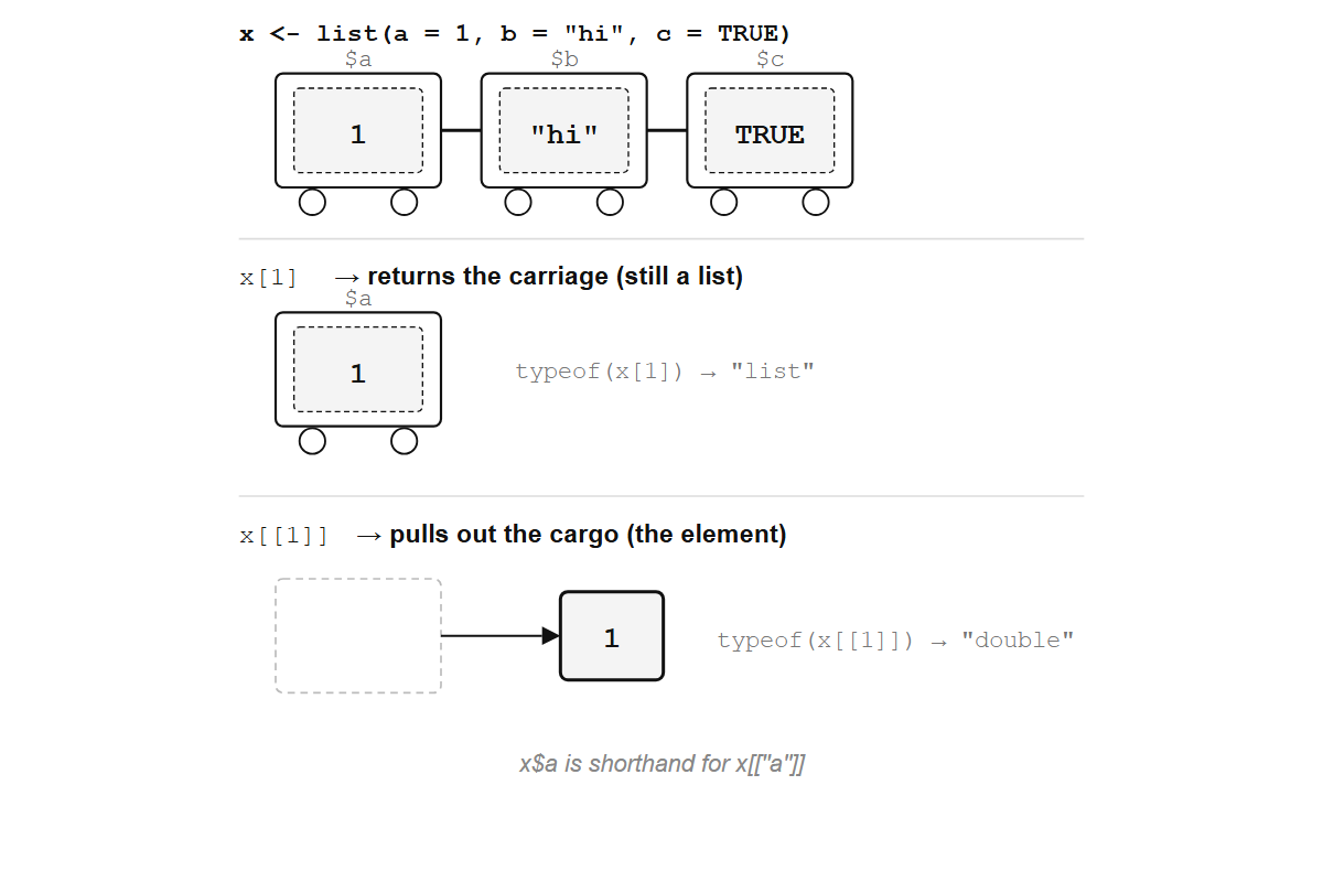
Figure 10.1: `x[1]` returns the carriage (still a list); `x[[1]]` pulls out the cargo (the element itself).

x <- list(a = 10, b = c(1, 2, 3), c = "hello")

[ returns a sub-list:

x[1]
#> $a
#> [1] 10
typeof(x[1])
#> [1] "list"

Still a list, just a shorter one.

[[ extracts the element:

x[[1]]
#> [1] 10
typeof(x[[1]])
#> [1] "double"

Now it’s the number 10, not a list containing 10. This distinction is the single most common source of confusion with lists: [ keeps the container, [[ removes it.

$ works with names:

x$b
#> [1] 1 2 3
x[["b"]]
#> [1] 1 2 3

Both return the same thing. $ is convenient for interactive use, but [[ is necessary when the name is stored in a variable:

key <- "b"
x[[key]]
#> [1] 1 2 3

x$key
#> NULL

x$key looks for a literal element named "key", not for the value stored in the variable key. Whenever the name is computed or passed as an argument, you need [[.

You can select multiple elements with [:

x[c(1, 3)]
#> $a
#> [1] 10
#> 
#> $c
#> [1] "hello"
x[c("a", "c")]
#> $a
#> [1] 10
#> 
#> $c
#> [1] "hello"

But [[ only works with a single index, extracting one element at a time.

Opinion

Default to [[ and $ for extracting elements. Use [ only when you need a sub-list. If you find yourself writing x[1][[1]], you wanted x[[1]] all along.

Exercises

Given x <- list(a = 10, b = 20, c = 30), predict the output of x[2], x[[2]], and x$b before running them.
What is typeof(x[1]) versus typeof(x[[1]])? Explain the difference.
Create a variable name <- "c". Use it to extract the element "c" from the list x. Which accessor works?

10.3 Nested lists

A list element can be another list, which means that a single list can grow into a tree of arbitrary depth:

study <- list(
  site = "Palmer Station",
  years = 2007:2009,
  species = list(
    list(name = "Adelie", count = 152),
    list(name = "Gentoo", count = 124),
    list(name = "Chinstrap", count = 68)
  )
)

str() reveals the shape:

str(study)
#> List of 3
#>  $ site   : chr "Palmer Station"
#>  $ years  : int [1:3] 2007 2008 2009
#>  $ species:List of 3
#>   ..$ :List of 2
#>   .. ..$ name : chr "Adelie"
#>   .. ..$ count: num 152
#>   ..$ :List of 2
#>   .. ..$ name : chr "Gentoo"
#>   .. ..$ count: num 124
#>   ..$ :List of 2
#>   .. ..$ name : chr "Chinstrap"
#>   .. ..$ count: num 68

str() is the single most useful function for lists. It works on any R object, but with lists it shows you the nesting, the types, and the lengths in one compact summary. Get in the habit of calling it on anything you did not build yourself.

Every nested list is a tree: sub-lists are branches, atomic values are leaves. File systems, the DOM, and JSON are all trees too, which is why R’s lists map onto them so naturally.

Inspecting is only half the problem. How do you reach into the tree and pull out what you need? Chain [[ or $:

study$species[[1]]$name
#> [1] "Adelie"
study[["species"]][[2]][["count"]]
#> [1] 124

Each [[ or $ steps one level deeper: study$species is a list of three lists, study$species[[1]] is the first of those, and study$species[[1]]$name is the string "Adelie". JSON from a web API, the output of lm(), and configuration files are all nested lists or objects built on them, and the access pattern is always the same: $ or [[ to step down one level, repeated as many times as needed.

Exercises

Given the study list above, extract the count for Chinstrap penguins.
Use str() on the result of lm(mpg ~ wt, data = mtcars). How many top-level elements does the model object have?
Create a nested list representing a book: title, author, and a list of chapters (each with a number and a title). Extract the title of the second chapter.

10.4 Lists as the backbone of R

You might think of lists as a container you reach for occasionally, but in truth they are the foundation that most of R’s familiar structures are built on.

A data frame is a list:

df <- data.frame(x = 1:3, y = c("a", "b", "c"))
typeof(df)
#> [1] "list"
is.list(df)
#> [1] TRUE

Each column is one element of that list, and the data frame simply adds a constraint: all columns must have the same length. Underneath, df$x works exactly like list access because it is list access.

A linear model is a list:

fit <- lm(mpg ~ wt, data = mtcars)
typeof(fit)
#> [1] "list"
names(fit)
#>  [1] "coefficients"  "residuals"     "effects"       "rank"         
#>  [5] "fitted.values" "assign"        "qr"            "df.residual"  
#>  [9] "xlevels"       "call"          "terms"         "model"

fit$coefficients, fit$residuals, fit$fitted.values — these are ordinary $ extractions on a list. The "lm" class attribute changes how R prints and summarizes the object, not how you get data out of it.

Data frames (Chapter 11), model objects, and environments are all lists (or list-like structures) with different rules about what they can contain. The most interesting rule is also the simplest: what happens when every element is a vector of the same length?

Exercises

Run typeof() on a data frame you create. Then run is.list() on it. What do you conclude?
Fit a model with lm(Sepal.Length ~ Petal.Length, data = iris). Use names() to see its elements, then extract the R-squared from summary() of the fit. (Hint: str(summary(fit)) will help.)
What does length() return for a data frame with 5 columns and 100 rows? Why?

10.5 Modifying lists

Adding an element is as simple as assigning to a new name:

x <- list(a = 1, b = 2)
x$c <- 3
x[["d"]] <- "new"
str(x)
#> List of 4
#>  $ a: num 1
#>  $ b: num 2
#>  $ c: num 3
#>  $ d: chr "new"

Removing an element means setting it to NULL:

x$b <- NULL
str(x)
#> List of 3
#>  $ a: num 1
#>  $ c: num 3
#>  $ d: chr "new"

b is gone, not set to NULL. This is a common trap: assigning NULL to a list element deletes it entirely. If you actually want to store NULL as a value, you need x["e"] <- list(NULL):

x["e"] <- list(NULL)
str(x)
#> List of 4
#>  $ a: num 1
#>  $ c: num 3
#>  $ d: chr "new"
#>  $ e: NULL

Now e exists and its value is NULL. The single-bracket assignment with list(NULL) is the only way to store an actual NULL in a list, an asymmetry worth memorizing because it bites everyone at least once.

Replacing an element is just assignment to an existing name:

x$a <- 100
x$a
#> [1] 100

R uses copy-on-modify for lists, the same semantics as for vectors. When you modify a list, R copies only the parts that change, not the entire structure; for practical purposes you can treat assignment as modifying in place, since the copying is an implementation detail that rarely affects your code.

Exercises

Create a list with elements x = 1 and y = 2. Add an element z = 3, then delete x. Print the result.
What does length() return after you delete an element from a list?
Try x$a <- NULL on a list where a exists. Then try x["a"] <- list(NULL). What is the difference?

10.6 Linked lists

R’s built-in lists are arrays of pointers, so indexing is O(1) and prepending is O(n) (every pointer in the array gets copied). A linked list is a chain of nodes, each holding a value and a pointer to the next. Prepending is O(1); reaching element k means following k pointers. You build one in R with nested lists:

cons <- function(head, tail) list(head = head, tail = tail)
car  <- function(lst) lst$head
cdr  <- function(lst) lst$tail

cons constructs a node, car extracts the first element, and cdr extracts the rest. These names come from Lisp (1958), where car and cdr referred to hardware registers on the IBM 704.

Build a linked list of three elements:

ll <- cons(1, cons(2, cons(3, NULL)))
str(ll)
#> List of 2
#>  $ head: num 1
#>  $ tail:List of 2
#>   ..$ head: num 2
#>   ..$ tail:List of 2
#>   .. ..$ head: num 3
#>   .. ..$ tail: NULL

To traverse it, recurse until you hit NULL:

ll_to_vector <- function(lst) {
  if (is.null(lst)) return(c())
  c(car(lst), ll_to_vector(cdr(lst)))
}
ll_to_vector(ll)
#> [1] 1 2 3

So why doesn’t R use linked lists for everyday work? Because R needs contiguous memory. Functions like sum() and the BLAS routines behind matrix algebra expect a single block of doubles that a C function can walk with a pointer, and a linked list scatters its elements across the heap (the region of memory where R allocates objects; Section 29.1 explains the distinction). R’s built-in lists (VECSXP) are arrays of pointers: O(1) random access, contiguous pointer storage. Linked lists trade that for O(1) prepend and natural recursive processing — peel off the head, recur on the tail. Lisp was built on that kind of processing; R was built on vectorized computation over contiguous arrays.

From Church encoding to cons cells

The cons/car/cdr structure is a direct translation of Church encoding. In lambda calculus, a pair is λh.λt.λf. f h t: a function that captures two values and waits for a selector. car passes a selector that returns the first value; cdr passes one that returns the second. A linked list is a chain of such pairs, terminated by a special “nil” value. Lisp was built on exactly this encoding, and cons/car/cdr remain the standard names for these operations across functional languages.

Both R and Lisp descend from the same lambda calculus, but the engineering decisions diverged early. Lisp committed to recursive decomposition: peel from the head, recur on the tail, build up an answer one cons at a time. R went the other way — contiguous arrays, vectorized operations, the C runtime walking a flat block of memory at speed. That fork propagated through every design decision that followed. R has sapply where Lisp has mapcar. R’s [ extracts by position; Lisp peels from the front. The entire language favors breadth over depth, and the linked list code above shows what depth-first design looks like from the inside.

Exercises

Using cons, car, and cdr defined above, build the linked list (10, 20, 30) and extract the second element without converting to a vector.
Write a function ll_length that counts the number of nodes in a linked list by recursing through cdr until NULL.
Write a function ll_map that takes a linked list and a function, and returns a new linked list with the function applied to each element. Test it by doubling every element of cons(1, cons(2, cons(3, NULL))).

10.7 Looking ahead

Lists hold anything, including other lists. Constrain that freedom (require every element to be a vector of the same length) and the general-purpose container becomes a table.