# Each c() call copies the entire existing vector
result <- c()
for (i in seq_len(n)) {
  result <- c(result, i)  # copies 1, then 2, then 3, ... elements
}
# Total copies: 1 + 2 + ... + n = n(n+1)/2 = O(n^2)9 Complexity and algorithms
You write a loop that takes three seconds on your test data. You deploy it on the full dataset, ten times larger, and it takes five minutes. Not thirty seconds. Five minutes. You double-check the code; nothing has changed, nothing is obviously wrong. The loop is doing the same thing it did before, just on more rows. So why did a 10x increase in data produce a 100x increase in running time?
The answer is not about your code being “bad,” and no amount of hardware will fix it. It is about the shape of growth: how running time scales with input size, and why some operations hit a wall that scales steeper than you expected. Big-O notation, hash tables, the limits of computation: these ideas draw the line between code that scales and code that chokes. They also explain why that line exists at all.
9.1 Not all operations are equal
Consider two ways to find a value in a vector. x[5] jumps directly to the fifth memory address, regardless of how long the vector is. which(x == 5) checks every element one by one until it finds a match. For a vector of length 10, you would not notice the difference. For a vector of length 10 million, you would.
A constant-time operation stays constant whether the input has ten elements or ten billion, while a linear operation scales proportionally, doing twice the work on twice the data. How running time scales with input size: that is the core idea of computational complexity, and once you see it, you start noticing it everywhere.
9.2 Big-O notation
Big-O notation makes this precise: we say f(n) is O(g(n)) if, past some input size, f grows no faster than a constant multiple of g.
The notation strips away constant factors and lower-order terms, which means an algorithm that takes 3n² + 100n + 7 steps is simply O(n²). The constants matter in practice (a factor of 10 is still a factor of 10), but Big-O captures the shape of growth, and that shape dominates once n gets large enough. When n is small, the constant factors dominate instead, and the algorithm with less overhead wins regardless of its Big-O.
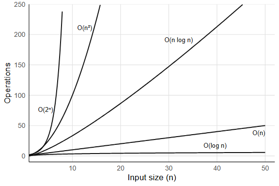
9.2.1 Common complexity classes
O(1): constant time. The operation takes the same time regardless of input size. length(x) is O(1) because R stores the length as an attribute and never counts the elements; indexing by position (x[5]) is also O(1), since R computes a memory offset and jumps directly to it. A less obvious example, and a more interesting one, is hash table lookup, which gets its own section below (Section 9.3).
O(log n): logarithmic time. Each step halves the search space. Binary search is the classic example: findInterval(0.5, sorted_x) finds where 0.5 falls in a sorted vector by repeatedly splitting it in half, which on a million elements takes roughly 20 comparisons and on a billion elements about 30. Logarithmic growth is extremely slow. So slow it barely registers.
O(n): linear time. You touch every element once. sum(x) walks the entire vector, adding each element: one pass, n additions. which(x > 0) also scans every element once, selecting those that match. Linear is often the best you can do, because you need to at least read all the input.
O(n log n): linearithmic time. The cost of sorting. sort(x) for a vector of length n makes O(n log n) comparisons, which is only slightly worse than linear: sorting a million numbers takes about 20x more work than summing them, not 1,000,000x more. Can you do better? For comparison-based sorting, no: there is a proof (via decision trees) that any algorithm which sorts by comparing pairs of elements must make at least O(n log n) comparisons in the worst case. Radix sort sidesteps this bound by not comparing elements at all (it distributes them into buckets by digit) but it only works when the keys have bounded range (integers, fixed-length strings).
O(n²): quadratic time. Nested loops where both loops run over the input. This is where performance falls apart. The classic R example is growing a vector with c():
Chapter 28 revisits this bottleneck in detail. The quadratic cost is not inevitable for append-style operations: if R used a doubling strategy (as Python’s list.append does), each individual append would be O(1) amortized. The idea is to allocate double the space when the array fills up; most appends just write to the next slot (O(1)), and the occasional O(n) resize happens rarely enough that the average cost per operation is constant. R does not do this for c(), which is why pre-allocation matters. A naive distance matrix computation is also O(n²): for n points, you compute n(n-1)/2 pairwise distances.
O(2^n): exponential time. Brute-force enumeration of all subsets. A set of n elements has 2^n subsets: at n = 20 that is about a million, at n = 30 a billion, at n = 50 over a quadrillion. Exponential algorithms are effectively unusable for large inputs, and no clever constant-factor tricks will save you.
9.2.2 How to tell empirically
The simplest test: double n and see what happens to the time. If the time roughly doubles, you have O(n); if it roughly quadruples, O(n²). Try this with sum(rnorm(n)) (linear) versus the c() growth loop (quadratic) for n = 1000, 2000, 5000, 10000. The ratio test works because Big-O captures the exponent, and doubling the input raises a power-law relationship to the surface. What happens when the ratio is somewhere between 2 and 4? A ratio near 2.8 when you double n suggests O(n^1.5), and in general a ratio of r implies a growth exponent of log2(r). You can also fit a log-log regression: plot log(time) against log(n), and the slope estimates the exponent directly.
Exercises
- What is the Big-O complexity of
rev(x)for a vector of length n? Why? - You have a sorted vector of length n. Compare the time of
x[1](get the minimum) versusmin(x)(scan for the minimum). What are their complexities? - The function
outer(x, y, "-")computes all pairwise differences between two vectors. If both have length n, what is the complexity in time and space?
9.3 Hash tables: O(1) lookup from scratch
Suppose you have a list of 10,000 names and you need to check whether "beta" is among them. The naive approach scans the list from the beginning, comparing each entry, and on average you check half the entries before finding a match (or all of them if the name isn’t there). That is O(n).
If the list is sorted, binary search gets you to O(log n). But there is a way to get O(1), constant time, regardless of how many names are in the list.
The trick is to turn the name into a number. A hash function takes a string (or any value) and produces an integer. For example, a simple hash might sum the character codes of each letter:
simple_hash <- function(key, n_slots) {
  codes <- utf8ToInt(key)
  (sum(codes) %% n_slots) + 1   # map to a slot between 1 and n_slots
}

simple_hash("beta", 10)
#> [1] 3
simple_hash("gamma", 10)
#> [1] 6
simple_hash("alpha", 10)
#> [1] 9
Now allocate a fixed-size array (say 10 slots). To store "beta" = 2, compute simple_hash("beta", 10) and put the value in that slot; to look it up later, compute the same hash, jump directly to that slot, and read the value. No scanning. The hash function converts a search problem into an arithmetic problem.
# Build a hash table by hand
n_slots <- 10
slots <- vector("list", n_slots)

# Insert three key-value pairs
insert <- function(slots, key, value, n_slots) {
  i <- simple_hash(key, n_slots)
  slots[[i]] <- list(key = key, value = value)
  slots
}

slots <- insert(slots, "alpha", 1, n_slots)
slots <- insert(slots, "beta",  2, n_slots)
slots <- insert(slots, "gamma", 3, n_slots)

# Look up "beta": one hash computation, one slot access
lookup <- function(slots, key, n_slots) {
  i <- simple_hash(key, n_slots)
  if (!is.null(slots[[i]])) slots[[i]]$value else NA
}

lookup(slots, "beta", n_slots)
#> [1] 2
One hash computation, one array access, O(1). That is the entire idea.
The problem is collisions: two different keys can hash to the same slot, and our simple_hash sums character codes, so any two strings with the same character-code sum will collide. When that happens, the slot needs to hold multiple entries, and the standard fix is chaining, where each slot stores a linked list of key-value pairs. On lookup, you hash to the slot, then scan the short list:
# A hash table with chaining
insert_chain <- function(slots, key, value, n_slots) {
  i <- simple_hash(key, n_slots)
  slots[[i]] <- c(slots[[i]], list(list(key = key, value = value)))
  slots
}

lookup_chain <- function(slots, key, n_slots) {
  i <- simple_hash(key, n_slots)
  chain <- slots[[i]]
  for (entry in chain) {
    if (entry$key == key) return(entry$value)
  }
  NA
}

slots2 <- vector("list", 10)
slots2 <- insert_chain(slots2, "alpha", 1, 10)
slots2 <- insert_chain(slots2, "beta",  2, 10)
slots2 <- insert_chain(slots2, "gamma", 3, 10)

lookup_chain(slots2, "beta", 10)
#> [1] 2
lookup_chain(slots2, "missing", 10)
#> [1] NA
In the worst case, every key hashes to the same slot, the chain has n entries, and lookup degrades to O(n). But a good hash function distributes keys evenly across slots, keeping each chain short: with n keys and n slots, the average chain length is 1, and lookup is O(1) on average.
R uses exactly this mechanism for environments. Every environment is a hash table mapping names to values, so when you write e$beta, R hashes the string "beta", jumps to the right slot, and returns the value. This is also why match(), duplicated(), %in%, unique(), and table() are fast: they build a temporary hash table internally, making membership tests O(1) per query instead of O(n).
# R environments are hash tables
e <- new.env(hash = TRUE, parent = emptyenv())
e$alpha <- 1
e$beta  <- 2
e$gamma <- 3

# This does NOT scan through "alpha" first.
# The hash of "beta" points directly to the right slot.
e$beta
#> [1] 2
The constant in O(1) depends on the hash function’s speed and the collision rate. Real hash functions (R uses one internally for its environments) are more sophisticated than summing character codes, distributing keys more uniformly and handling edge cases. But the principle is always the same: convert the key to an integer, use it as an index, handle collisions with chaining.
What happens when the table fills up? The chains get longer, and lookup degrades toward O(n). Real hash tables track the load factor (number of entries divided by number of slots) and resize, typically doubling the slot count, when it crosses a threshold (often 0.75). Resizing costs O(n) because every key must be rehashed into the new array, but it happens rarely enough that the amortized cost per insertion stays O(1).
Exercises
- What happens to
simple_hashif two keys have the same character-code sum? Trysimple_hash("ab", 10)andsimple_hash("ba", 10). Why is this a problem, and how does chaining solve it? - Our hand-built hash table has a fixed number of slots. What happens as you insert many more keys than slots? How does the average chain length change? (This is why real hash tables resize: when the load factor exceeds a threshold, they allocate a larger array and rehash all keys.)
- Use
system.time()to comparex %in% yversus a loop withany(y == x[i])forx <- sample(1e6)andy <- sample(1e4). The first builds a hash table; the second does linear scans.
9.4 Space complexity
Time is not the only resource that scales. Memory matters too, especially in R where data frames can be gigabytes, and running out of RAM kills your session more decisively than a slow loop ever could.
A full copy of a 1 GB data frame uses 1 GB of additional memory; two copies and you are at 3 GB total. R’s garbage collector reclaims unused memory, but if multiple large objects are live simultaneously, you can exhaust RAM. How does R decide when to copy?
9.4.1 Copy-on-modify
R uses copy-on-modify semantics: when you assign an object to a new name, R does not immediately copy it. Both names point to the same underlying data, and a copy is triggered only when one reference is modified:
x <- rnorm(1e6)
y <- x              # no copy yet: x and y share the same memory
y[1] <- 0           # NOW R copies the entire vector, then modifies element 1
You can verify this with lobstr::obj_addr():
library(lobstr)
x <- rnorm(1e6)
y <- x
obj_addr(x) == obj_addr(y)  # TRUE: same memory

y[1] <- 0
obj_addr(x) == obj_addr(y)  # FALSE: y is now a separate copy
Copy-on-modify is why passing large objects to functions is cheap in R: the function receives a reference, not a copy, and a copy happens only if the function modifies the object. But when modification does happen (say, inside a loop) the cost can compound quickly, turning what looks like an O(n) operation into something much worse.
9.4.2 Pre-allocation vs. growing
The c() loop from the quadratic example above is slow in time and wasteful in memory. Each iteration allocates a new vector of size i, copies the old data, and discards the old allocation, so the total memory allocated across all iterations is 1 + 2 + 3 + … + n = O(n²), even though the final result uses only O(n) space.
Pre-allocation fixes both problems:
# O(n²) total memory allocated
result <- c()
for (i in seq_len(n)) result <- c(result, i)

# O(n) total memory allocated
result <- numeric(n)
for (i in seq_len(n)) result[i] <- i
9.4.3 Measuring memory
x <- rnorm(1e6)
object.size(x)
#> 8000048 bytes
object.size() gives a rough estimate. For more accurate measurements, including shared memory between objects:
lobstr::obj_size(x)

# Shared memory: two references to the same object
y <- x
lobstr::obj_size(x, y)  # same as obj_size(x), not double
Exercises
- Create a list of 10 data frames, each with 1000 rows and 5 columns. Use
lobstr::obj_size()to measure the total. Is it 10 times the size of one data frame? - Explain why
x <- 1:1e8uses far less memory thanx <- as.numeric(1:1e8). (Hint: check withobject.size(). R stores the compact sequence as just a start, end, and step, exploiting the structure. This connects to Kolmogorov complexity: the shortest program that produces a given output. “Random” data is incompressible, while structured data likerep(1, 1e6)can be described in a few bytes. Compression algorithms approximate Kolmogorov complexity from above.) - Write a function that takes a data frame and returns it unchanged. Use
lobstr::obj_addr()to verify that no copy is made.
9.5 Common algorithms in R
You rarely implement algorithms from scratch in R, but the built-in functions make algorithmic choices on your behalf, and knowing what they chose helps you predict when they will be fast and when they will not.
9.5.1 Sorting
sort() uses a hybrid introsort: quicksort for the fast average case, switching to heapsort if quicksort degrades, and insertion sort for small sub-arrays. Worst-case time is O(n log n).
order() returns the permutation that would sort the vector, also O(n log n), and for data frames it is the basis of dplyr::arrange(). R also offers sort(x, method = "radix") for integer and character vectors; radix sort is O(n) for bounded-range integers, which is why data.table::setorder() is fast.
9.5.2 Searching and matching
match() and %in% build a hash table from one vector, then probe it for each element of the other. Building the table is O(n); each lookup is O(1) on average, so x %in% y is O(n + m) where n and m are the lengths of x and y.
findInterval() does binary search on a sorted vector: O(log n) per query. If you have many queries against the same sorted vector, findInterval can be faster than building a hash table, because the sorted structure is already there and hashing has overhead.
9.5.3 Hashing
duplicated(), unique(), and table() all use hash tables internally. That is why duplicated(x) is O(n), not the O(n²) you would get from comparing every pair of elements.
9.5.4 String matching
grep() and grepl() compile the pattern into a finite automaton, then scan the input strings. For fixed strings, fixed = TRUE skips regex compilation entirely:
# Regex: compiles pattern, then scans
grep("item_5", x)

# Fixed string: faster, no regex overhead
grep("item_5", x, fixed = TRUE)
For repeated matching against the same pattern, pre-compiling with stringi::stri_detect_regex() avoids recompilation.
Exercises
- You need to check whether each element of a vector
x(length 1 million) appears in a lookup tabley(length 100). Comparex %in% ywith a loop usingany(y == x[i]). What are their complexities? - Why is
duplicated(x)faster thanlength(unique(x)) < length(x)for simply checking whether duplicates exist? (Hint:duplicatedcan short-circuit in principle, though R’s implementation does not.) - You have a sorted numeric vector of length 10 million. You need to find where 1000 query values fall. Compare
findInterval(queries, sorted_vec)withmatch(queries, sorted_vec). Which is appropriate here, and why?
9.6 Computability
Everything above assumes the problem can be solved, that some algorithm exists, however slow, that will eventually produce the answer. Not all problems have that property.
9.6.1 The halting problem
By the early twentieth century, mathematicians had been on a winning streak that stretched back decades. Cantor had tamed infinity. Frege had formalized logic. Peano had reduced arithmetic to five axioms. Every time someone asked “can we make this rigorous?” the answer had been yes.
David Hilbert had watched this happen for thirty years, and in 1928 he posed the question that felt like the natural finish line: the Entscheidungsproblem, the decision problem. Could you build a mechanical procedure that takes any mathematical statement and tells you whether it is true or false? If such a procedure existed, mathematical truth would be computable. Every conjecture decidable, every proof checkable by turning a crank, but then in 1936 a twenty-three-year-old graduate student would shock the whole mathematical worldview.
He proved that no algorithm can decide, for an arbitrary program and input, whether that program will eventually halt or run forever. It was Alan Turing, the same graduate student whose tape machine we met in Section 1.1, now proving that his own machine had a boundary it could never cross.
The specific question he settled is called the halting problem. The proof is one of the most beautiful arguments in mathematics, it fits in half a page, and it works by turning the assumption against itself. We give it in full, twice: once in R and once in lambda calculus.
The proof by contradiction (in R). Assume, for the sake of contradiction, that a function halts(f, x) exists. It takes any function f and any input x, and returns TRUE if f(x) terminates, FALSE if f(x) runs forever. It always returns one or the other; it never crashes or loops itself. That is the assumption we will break.
Given halts, define a new function:
trouble <- function(x) {
  if (halts(trouble, x)) {
    while (TRUE) {}   # loop forever
  } else {
    return(x)          # halt
  }
}
Now ask: does trouble(trouble) halt?
Case 1: Suppose halts(trouble, trouble) returns TRUE. Then trouble(trouble) enters the if branch and loops forever. But halts said it would halt. Contradiction.
Case 2: Suppose halts(trouble, trouble) returns FALSE. Then trouble(trouble) enters the else branch and returns trouble. It halts. But halts said it would not. Contradiction.
Both cases contradict the assumption, and there is no third case (we assumed halts always returns TRUE or FALSE). Therefore halts cannot exist. No algorithm, in any language, can solve the halting problem for arbitrary programs.
The argument is a diagonal argument, the same technique Cantor used in 1891 to prove that the real numbers are uncountable, and the same structure Godel used in 1931 for the incompleteness theorems. The trick is always the same: assume a complete listing (or decision procedure) exists, then construct something that disagrees with every entry on the diagonal.
The proof in lambda calculus. Seeing the same proof in lambda calculus is worth the detour, because it shows that undecidability is not a quirk of loops or mutable state or any particular language’s execution model. The result falls out of self-application alone, which means it holds for any system powerful enough to pass functions to functions — R included.
Church proved the same result independently in 1936, before Turing’s paper, using the lambda calculus rather than a machine model. The argument has the same shape but uses different language.
In lambda calculus, every value is a function and every computation is function application. There are no loops; non-termination means a term reduces forever without reaching a normal form. For instance, the term (λx. x x)(λx. x x) applies itself to itself, producing the same term again, endlessly, never halting. This term is called Ω.
Church’s question: is there a lambda term H that, given any term M, returns true if M has a normal form (halts) and false if M reduces forever?
Assume H exists. Define:
D = λm. if (H (m m)) then Ω else Iwhere Ω is the non-terminating term from above and I = λx. x is the identity (which halts immediately). Now apply D to itself:
- If H(D D) returns
true(meaning D D halts), then D D reduces to Ω and loops forever. Contradiction. - If H(D D) returns
false(meaning D D diverges), then D D reduces to I and halts. Contradiction.
Same diagonal structure, same conclusion: H cannot exist. No lambda term can decide whether an arbitrary term has a normal form.
The mechanism that breaks H is self-application: a term applied to itself. That mechanism is not exotic. When you write function(f) f(f) in R, you are writing self-application. When you pass a function to sapply, you are handing a value to a function that will call it, one step from the same recursive knot. R has the same capability: functions are values, values can be passed to functions, and nothing prevents a function from receiving itself. Closures, recursion, and higher-order functions all depend on that freedom. The halting problem is the price.
Any language expressive enough to let functions consume themselves is expressive enough to construct the diagonal argument, and that includes every language in this book’s lineage from Lisp onward. When a linter warns you about unreachable code or an optimizer tries to eliminate dead branches, it is working inside the limits Church proved in 1936: necessarily incomplete, always capable of missing something.
Church published this in April 1936 (“An Unsolvable Problem of Elementary Number Theory”); Turing published his version in November 1936 (“On Computable Numbers”). They later proved that their two formalisms, lambda calculus and Turing machines, compute exactly the same class of functions. The halting problem is not an artifact of one model. It is a boundary.
Why it matters in practice. Rice’s theorem (1953) generalizes the result: any non-trivial semantic property of programs is undecidable. You cannot write a program that decides whether another program is “correct,” “efficient,” or “pure.” Tools like lintr and mypy use sound overapproximations, rejecting some correct programs to guarantee they never accept an incorrect one. The question is not whether your analyzer has blind spots, but where.
9.6.2 Practical workarounds
You cannot solve the halting problem in general, but you can set time limits:
# setTimeLimit: kill a computation after 5 seconds
setTimeLimit(elapsed = 5, transient = TRUE)
tryCatch(
  {
    # potentially non-terminating computation
    result <- some_function(x)
  },
  error = function(e) message("Computation timed out")
)
setTimeLimit(elapsed = Inf)  # reset
The R package R.utils provides withTimeout() for a cleaner interface. These are engineering solutions to a mathematically unsolvable problem: you cannot know whether the computation will finish, but you can decide how long you are willing to wait.
9.6.3 The Church-Turing thesis
Church and Turing proved that their two formalisms, lambda calculus and Turing machines, compute exactly the same class of functions (Section 9.6.1). The Church-Turing thesis states that any function computable by an effective procedure can be computed by a Turing machine, or equivalently, expressed as a lambda calculus term.
This has a concrete consequence: R, Python, C, Haskell, and every other general-purpose language can compute exactly the same set of functions. No language can solve the halting problem; no language can compute a function that another general-purpose language cannot. The differences between languages are speed, expressiveness, and safety, not computational power.
R’s functional core (functions as values, closures, recursion) is directly descended from lambda calculus, so when you write function(x) x + 1, you are writing a lambda term. The equivalence means R’s functional style and C’s imperative loops are two notations for the same mathematics.
9.6.4 P vs NP
Some problems are easy to verify but (probably) hard to solve. Given a proposed solution to the traveling salesman problem, you can check its total distance in O(n), but finding the optimal solution appears to require exponential time.
The class P contains problems solvable in polynomial time; the class NP contains problems whose solutions can be verified in polynomial time. Whether P = NP is the most famous open question in computer science, and most researchers believe P ≠ NP, which would mean some problems are fundamentally harder to solve than to check.
The subset sum problem makes the gap concrete. Given a set of integers, does any subset sum to a target value? Verifying a proposed subset is O(n), just add the numbers. Finding one by brute force means checking all 2^n subsets:
# Brute force: check all 2^n subsets (exponential)
subset_sum_brute <- function(x, target) {
  n <- length(x)
  for (i in seq_len(2^n) - 1) {
    bits <- as.logical(intToBits(i)[seq_len(n)])
    if (sum(x[bits]) == target) return(x[bits])
  }
  NULL
}

# A greedy approximation: sort descending, take what fits (polynomial)
subset_sum_greedy <- function(x, target) {
  x <- sort(x, decreasing = TRUE)
  picked <- logical(length(x))
  remaining <- target
  for (i in seq_along(x)) {
    if (x[i] <= remaining) {
      picked[i] <- TRUE
      remaining <- remaining - x[i]
    }
  }
  if (remaining == 0) x[picked] else NULL
}
At n = 20 the brute-force version checks about a million subsets and finishes in under a second. At n = 40 it checks a trillion — you will not wait long enough. The greedy version runs in O(n log n) on either input but is not guaranteed to find a solution that exists. That is the P-vs-NP gap in miniature: polynomial verification, (apparently) exponential search, and a fast heuristic that trades correctness for speed.
In practice, R encounters NP-hard problems in optimization. optim() does not guarantee a global optimum for non-convex problems; it uses heuristic methods (Nelder-Mead, simulated annealing) that find good-enough solutions without exhaustive search. This is the pragmatic response to intractability: give up on perfection and settle for “good enough, fast.”
The loop from the opening, the one that took five minutes instead of thirty seconds — you now have the vocabulary to diagnose it: somewhere in that loop, an O(n²) operation was hiding inside what looked like O(n) code, and the 10x increase in data exposed the quadratic scaling that small test sets had concealed. The growth rate was there from the start; faster hardware only postpones when you hit it.
But complexity is only half the story — the other half is the data structure you choose to hold your values, and so far the only container you have is the atomic vector, which insists that everything inside it be the same type.
Exercises
- Write a function that takes another function
fand an argumentx, callsf(x)with a 2-second time limit, and returnsNAif the computation does not finish. - Can a program determine whether a given R function is pure (no side effects)? Why or why not?
- Is sorting in P or NP? What about finding the shortest path that visits all cities exactly once (traveling salesman)?