4 Vectors

Type 42 in R.

42
#> [1] 42

That [1] has been there since Chapter 1, quietly announcing something you probably didn’t notice: you never made a number. You made a vector.

4.1 There are no scalars

In C or Python, a single number and a collection of numbers are fundamentally different types: one is a scalar, the other is an array or list. R erases that distinction. Every value in R is a vector: 42 is a numeric vector of length 1, "hello" is a character vector of length 1, and TRUE is a logical vector of length 1.

length(42)
#> [1] 1
length("hello")
#> [1] 1
length(TRUE)
#> [1] 1

Why would a language erase the distinction between “one thing” and “many things”? Because S (Section 2.3), the language R descends from, was built for people who work with columns of data, not individual numbers. A single temperature reading is rarely interesting on its own; you care about the whole column. So S made the column the basic unit of computation, and R inherited that decision wholesale, which means every operation you write, from arithmetic to comparison, has to reckon with that choice.

x * 2 works the same whether x has one element or a million, because x is always a vector and R doesn’t need a special case for scalars; it just operates on vectors. But how do you build them?

4.2 Atomic vectors

You make a vector with c(), short for “combine”:

temperatures <- c(72, 85, 61, 90, 78)
temperatures
#> [1] 72 85 61 90 78

c() can combine vectors too:

morning <- c(58, 62, 55)
afternoon <- c(75, 80, 71)
all_temps <- c(morning, afternoon)
all_temps
#> [1] 58 62 55 75 80 71

It flattens everything into a single vector; there are no nested vectors in R, so c(c(1, 2), c(3, 4)) gives you c(1, 2, 3, 4). Look at what’s happening in c(morning, afternoon):

c(morning, afternoon)
= c(c(58, 62, 55), c(75, 80, 71))
= c(58, 62, 55, 75, 80, 71)
= [58, 62, 55, 75, 80, 71]

Each step replaces a name or function call with its value. morning becomes c(58, 62, 55), the nested c() calls flatten into one, and the last step is where term replacement ends and the computer takes over: R allocates a contiguous block of memory, stores six numbers side by side, and the expression has been reduced to a value that lives in memory. This is term replacement, the logic at the heart of Church’s lambda calculus (Section 1.2): you have an expression, you replace each piece with its value until nothing is left to replace. In Chapter 1, add(3, add(5, 10)) reduced step by step until only 18 remained. Here, c(morning, afternoon) reduces to a six-element vector. Even building a data structure is a function call that reduces to a value. (Term replacement is one of the oldest ideas in logic and a cornerstone of computer science. Mathematicians were studying it decades before electronic computers existed; it turns out that “replace an expression with its value” is enough to define all of computation.)

For the curious

c() has two properties worth noticing. First, it is associative: c(c(1, 2), c(3, 4)) and c(1, c(2, c(3, 4))) both produce c(1, 2, 3, 4). Grouping doesn’t matter. Second, c(x, NULL) returns x unchanged, so NULL acts as an identity element: combining with it does nothing. An operation that is associative and has an identity element is called a monoid. Addition with 0 is a monoid. String concatenation with "" is a monoid. c() with NULL is a monoid. The pattern keeps showing up: dplyr pipelines (Chapter 14), function composition (Chapter 15), and Reduce() (Chapter 21) all rely on it.

A few shortcuts for common patterns:

1:5
#> [1] 1 2 3 4 5

seq(0, 1, by = 0.25)
#> [1] 0.00 0.25 0.50 0.75 1.00

rep("hello", 3)
#> [1] "hello" "hello" "hello"

1:5 generates integers from 1 to 5, seq() generates a sequence with a specified step size, and rep() repeats a value.

R has four atomic types you will use constantly, and every one of them follows a pecking order that R enforces behind your back. Two more exist but rarely matter:

typeof(3.14)
#> [1] "double"
typeof(42L)
#> [1] "integer"
typeof("hello")
#> [1] "character"
typeof(TRUE)
#> [1] "logical"

double is a decimal number (even 42 is stored as a double by default), while integer needs an L suffix: 42L. character is text, logical is TRUE or FALSE. The other two types, complex and raw, exist for specialized work; you can ignore them.

Every element in a vector must be the same type. typeof() and length() answer the two most basic questions about any vector: what type are the elements, and how many are there? But what happens when you try to break that same-type rule?

Exercises

What does c(1, c(2, c(3, 4))) produce? Predict, then check.
Create a vector of the first 10 even numbers using seq().
What is typeof(1)? What about typeof(1L)?

4.3 Coercion

Try mixing types in a vector:

c(1, "two", 3)
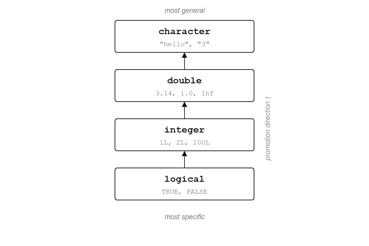
#> [1] "1"   "two" "3"

R converted the numbers to text. No warning, no error. This is called coercion, and R follows a fixed hierarchy: logical < integer < double < character. When you mix types, everything gets promoted to the most general one.

c(TRUE, 1, "hello")
#> [1] "TRUE"  "1"     "hello"

TRUE became "1" (first promoted to the integer 1, then to the string "1"), and 1 became "1".

This hierarchy explains a trick from Chapter 1 that might have seemed like magic. sum(scores > 70) works because scores > 70 produces a logical vector, and sum() coerces the logicals to numbers: TRUE becomes 1, FALSE becomes 0, so the count of passing values falls out automatically:

x <- c(65, 82, 71, 90, 55, 78)
x > 70
#> [1] FALSE  TRUE  TRUE  TRUE FALSE  TRUE
sum(x > 70)
#> [1] 4

Opinion

R will never warn you about coercion. c(1, 2, "3") quietly becomes all character, and your arithmetic breaks ten lines later with an error message that points nowhere near the real problem. Memorize the hierarchy: logical < integer < double < character. It will save you hours.

Figure 4.1: R’s coercion hierarchy: mixing types promotes everything to the most general type.

Exercises

What does TRUE + 1 return? What about FALSE * 5?
What is typeof(c(1L, 1.5))? Which type won?
What does as.numeric("hello") return? Read the warning.

4.4 Vectorized operations

Say you have five temperatures in Fahrenheit and want Celsius. In most languages, you write a loop: go through each element, apply the formula, store the result. In R:

temperatures <- c(72, 85, 61, 90, 78)
(temperatures - 32) * 5/9
#> [1] 22.22222 29.44444 16.11111 32.22222 25.55556

One expression, no loop. The subtraction, multiplication, and division each apply to every element at once. This is a vectorized operation, and it is the default way of working in R.

Comparisons are vectorized too:

temperatures > 75
#> [1] FALSE  TRUE FALSE  TRUE  TRUE

The result is a logical vector of the same length: TRUE where the condition holds, FALSE where it doesn’t.

You can combine comparisons with & (and) and | (or):

temperatures > 60 & temperatures < 85
#> [1]  TRUE FALSE  TRUE FALSE  TRUE

Arithmetic, comparisons, and most built-in functions all work this way, returning a vector of the same length for each input vector. sqrt(), log(), round(), abs(): give them a vector and they return a vector.

sqrt(c(1, 4, 9, 16, 25))
#> [1] 1 2 3 4 5

In lambda calculus (Section 1.2), sqrt is a function f = λx. √x. Even √ itself is not a primitive; it can be computed by repeated function application. You start with a rough guess and improve it over and over until it’s close enough:

√x = iterate(λguess. (guess + x / guess) / 2, x)

Start with a guess, apply the refinement function λguess. (guess + x / guess) / 2 repeatedly, and the result converges to √x. Square root reduces to division, addition, and repeated application of a lambda, which are themselves reducible further. At every level, the building blocks are functions applied to arguments.

Under the hood

In practice, R calls C’s sqrt(), which on modern CPUs maps to a hardware instruction. The chip uses a lookup table for a rough estimate, then refines it with the same (guess + x / guess) / 2 step, finishing in 10-20 clock cycles. The abstraction and the silicon converge on the same algorithm.

For our purposes, f = λx. √x is enough. R applies f to each element by term replacement:

f = λx. √x

f(c(1, 4, 9, 16, 25))
= c(f(1), f(4), f(9), f(16), f(25))          # distribute f over the vector
= c((λx. √x)(1), (λx. √x)(4), ..., (λx. √x)(25))  # replace f with its definition
= c(√1, √4, √9, √16, √25)                   # substitute each x
= c(1, 2, 3, 4, 5)

R distributes the function over the vector automatically; you write one application, R performs five. This is Church’s model extended to collections: a function applied to a vector produces a vector of results. sqrt(c(1, 4, 9, 16, 25)) is a single function applied to a single argument, and the fact that the argument contains five numbers is R’s business, not yours.

For the curious

This pattern has a name: a functor. A functor maps a function over a structure while preserving the structure’s shape. sqrt applied to a five-element vector returns a five-element vector; the function changes the contents, but the container stays intact. Vectors are functors, lists are functors (via lapply), and data frame columns are functors (via mutate). The word comes from category theory, but the idea is concrete: apply inside, preserve outside. You will see it everywhere in this book, and by the end it will feel as natural as vectorization itself.

Consider what temperatures * 9/5 + 32 actually did. A function was applied to a structure and produced a structure of the same shape — a functor operation, driven by the same term-replacement mechanism that Section 1.2 introduced as lambda calculus. And when you wrote c(morning, afternoon), the names were substituted for their values and the expression reduced to a single vector. That is beta reduction: replacing a name with its value and simplifying (Section 1.2 covers the formal version). The theoretical machinery from Chapter 1 has been running under every line of code in this chapter, not as background context but as the engine. By the time you typed 42 into the console and got 42 back, you were already doing functional programming — you just did not have a name for it yet.

4.4.1 Recycling

What happens when you operate on two vectors of different lengths?

c(1, 2, 3, 4) + c(10, 20)
#> [1] 11 22 13 24

R recycled the shorter vector, reusing 10, 20 to match the length of the longer one: 1+10, 2+20, 3+10, 4+20. This is also how temperatures - 32 works: 32 is a vector of length 1, and R recycles it five times to match the length of temperatures.

When the lengths don’t divide evenly, R warns you:

c(1, 2, 3, 4, 5) + c(10, 20)
#> Warning in c(1, 2, 3, 4, 5) + c(10, 20): longer object length is not a
#> multiple of shorter object length
#> [1] 11 22 13 24 15

Opinion

Recycling is useful when the shorter vector has length 1 (e.g., x * 2, x > 0). For anything else, match your vector lengths explicitly. A recycling warning almost always means a bug.

Exercises

What does c(1, 2, 3) * c(0, 1) produce? Does R warn you?
Why does x - mean(x) work without a loop? (Hint: what length is mean(x)?)
What does c(TRUE, FALSE) + c(1, 2, 3, 4) produce?

4.5 Indexing

You often need specific elements from a vector, and the [ operator extracts them. There are four ways to use it.

By position:

temperatures <- c(72, 85, 61, 90, 78)
temperatures[1]
#> [1] 72
temperatures[c(1, 3, 5)]
#> [1] 72 61 78

By exclusion (negative indices):

temperatures[-2]
#> [1] 72 61 90 78

Everything except the second element.

By logical vector:

temperatures[temperatures > 75]
#> [1] 85 90 78

temperatures > 75 produces c(FALSE, TRUE, FALSE, TRUE, TRUE), and [ keeps only the TRUE elements. You’re asking a yes/no question of every element and keeping the ones that pass. This is filtering, and it will come back in a more powerful form when you learn dplyr::filter() (Chapter 14).

hot <- temperatures > 75
temperatures[hot]
#> [1] 85 90 78

By name:

scores <- c(alice = 92, bob = 78, carol = 85)
scores["bob"]
#> bob 
#>  78
scores[c("alice", "carol")]
#> alice carol 
#>    92    85

You can also use [ to replace elements:

x <- c(10, 20, 30)
x[2] <- 99
x
#> [1] 10 99 30

This looks like it’s changing the vector in place, but R is actually making a copy with the new value and pointing the name x at the copy. The old vector (with 20 in position 2) is gone. This is copy-on-modify, the same idea from Section 3.2: values in R don’t change; names get moved to point at new values. So far, every element in our vectors has been present and accounted for, but real data has gaps.

Exercises

Extract the last element of temperatures without hard-coding the position. (Hint: length().)
What does temperatures[c(TRUE, FALSE)] return? How does recycling interact with logical indexing?
Create a named vector of three cities and their populations. Extract two by name.

4.6 Missing values

A sensor fails, a patient skips a visit, a field is left blank. Real data has gaps, and R represents them with NA (“Not Available”):

readings <- c(23.1, NA, 22.5, 24.0, NA, 23.8)
readings
#> [1] 23.1   NA 22.5 24.0   NA 23.8

NA is not zero, and it is not an empty string. It means “I don’t know.” And that uncertainty is contagious: any computation involving an unknown value produces an unknown result.

sum(readings)
#> [1] NA
mean(readings)
#> [1] NA

R is being honest. If you don’t know some of the values, you don’t know the sum. If you want to ignore the missing values, you have to say so explicitly:

sum(readings, na.rm = TRUE)
#> [1] 93.4
mean(readings, na.rm = TRUE)
#> [1] 23.35

na.rm = TRUE means “remove NAs before computing.” Many R functions have this argument.

Find which elements are missing with is.na():

is.na(readings)
#> [1] FALSE  TRUE FALSE FALSE  TRUE FALSE

Filter them out with ! (not):

readings[!is.na(readings)]
#> [1] 23.1 22.5 24.0 23.8

One common trap: you cannot test for NA with ==.

NA == NA
#> [1] NA

This returns NA, not TRUE. Think about it: if you don’t know what x is and you don’t know what y is, you can’t know whether they’re equal. Always use is.na().

This contagious behavior is not arbitrary; R is implementing a discipline where a value is either present or absent, and any operation on an absent value produces absence. The principle is older than R.

Haskell, a language that emerged in 1990 when a group of functional programming researchers decided to consolidate their dozens of incompatible dialects, takes the strictest possible position: no variable can ever change its value, and no function can have a side effect. The compiler enforces these rules, which means the type system carries more information than in most languages. (The language is named after Haskell Curry, a logician who worked on combinatory logic in the 1930s and 1940s; he will reappear in Section 5.8.)

One consequence: in Haskell, the possibility of absence is built into the type system as Maybe. A value is either Just 42 or Nothing, and any operation on Nothing propagates Nothing forward. 1 + NA returning NA in R is the same logic as Haskell’s Nothing >>= f returning Nothing.

Rust adopted the same idea for different reasons. Graydon Hoare started Rust at Mozilla in 2006 because C and C++ gave you direct control over memory but no protection against the bugs that come with it: buffer overflows, use-after-free, data races. He borrowed heavily from Haskell’s type system, and Rust’s equivalent of Maybe is called Option: a value is Some(42) or None, and None.map(f) returns None. The compiler rejects any code that forgets to check whether a value is present.

R’s approach is looser: nothing stops you from ignoring NA, and you will not find out until your results look wrong. But the underlying rule is the same. If any input is unknown, the output is unknown. R threads this uncertainty through every arithmetic and comparison operation automatically, which is why NA feels contagious. It is. That’s the point. The question is what this contagion looks like when you have 344 measurements and a handful of gaps.

Exercises

What does c(1, NA, 3) > 2 return? What happens to the NA?
How many missing values are in readings? (Hint: combine sum() and is.na().)
What does NA | TRUE return? What about NA & FALSE? One of each pair is not NA. Why?

4.7 Meet penguins

R 4.5 and later includes a dataset called penguins (from the Palmer Archipelago in Antarctica), and it’s a good place to see everything from this chapter working on real measurements. If you’re running an older version, install it with install.packages("palmerpenguins") and load it with library(palmerpenguins).

head(penguins)

penguins is a data frame (a table), and we’ll learn about those properly in Chapter 11. For now, the important thing is that you can pull out a single column with $, and that column is a vector:

bill <- penguins$bill_length_mm

Now you have a numeric vector of 344 bill length measurements, with some NAs mixed in. Everything from this chapter applies:

length(bill)
typeof(bill)

mean(bill, na.rm = TRUE)
range(bill, na.rm = TRUE)

sum(is.na(bill))

long_bills <- bill[bill > 50 & !is.na(bill)]
length(long_bills)

How many penguins have a bill longer than 50 mm? Logical indexing filters the values, is.na() handles missing data, and length() counts the result. One line each, no loops. You wrote five operations in this chapter that would each require explicit iteration in most languages; in R, the vector carried the iteration for you. Data frames, which we turn to next, are built from exactly these vectors, stacked side by side like columns in a spreadsheet. The machinery you just learned doesn’t go away; it becomes the engine underneath everything else.

Exercises

What is the mean body mass (penguins$body_mass_g) of the penguins? Don’t forget the NAs.
How many penguins have a flipper length (penguins$flipper_length_mm) greater than 200?
What is the shortest bill in the dataset? (Hint: min() with na.rm = TRUE.)