12 Strings, factors, and dates

Numbers are easy. Text, categories, and dates are where data gets messy. This chapter groups three types of data that look simple but hide complexity: strings (text that needs parsing, matching, and cleaning), factors (categories that need ordering and recoding), and dates (time values that need arithmetic and formatting). Each has a dedicated tidyverse package (stringr, forcats, lubridate), and each comes with traps that catch beginners. This chapter gives you enough to be productive, not exhaustive.

We will use the palmerpenguins dataset throughout. Load it now:

library(palmerpenguins)
#> 
#> Attaching package: 'palmerpenguins'
#> The following objects are masked from 'package:datasets':
#> 
#>     penguins, penguins_raw
library(stringr)
library(forcats)
library(lubridate)
#> 
#> Attaching package: 'lubridate'
#> The following objects are masked from 'package:base':
#> 
#>     date, intersect, setdiff, union

12.1 Character vectors

A string in R is a character vector of length 1. "hello" is not a special string type; it is character(1), the same kind of atomic vector you met in Section 4.2.

x <- "hello"
typeof(x)
#> [1] "character"
length(x)
#> [1] 1

Double quotes and single quotes both work. Pick one and be consistent.

Opinion

Use double quotes. R’s own style guide does. Most code you will read does. Single quotes are fine inside double-quoted strings: "it's easy".

R uses UTF-8 as its modern string encoding, an encoding that Ken Thompson and Rob Pike designed on a placemat in a New Jersey diner in September 1992. UTF-8 is backward-compatible with ASCII, self-synchronizing, and variable-width (one to four bytes per character). When accented characters turn to garbled text, stringr::str_conv() or readr::locale(encoding = "latin1") will fix it.

Special characters use backslash escapes: \n (newline), \t (tab), \\ (literal backslash). The difference between print() and cat() matters here:

print("line one\nline two")
#> [1] "line one\nline two"
cat("line one\nline two")
#> line one
#> line two

print() shows the escape sequence as text. cat() renders it.

Base R provides a handful of string tools:

nchar("penguin")
#> [1] 7
paste("Gentoo", "penguin")
#> [1] "Gentoo penguin"
paste0("Gentoo", "penguin")
#> [1] "Gentoopenguin"
sprintf("The %s weighs %d grams", "Gentoo", 5200)
#> [1] "The Gentoo weighs 5200 grams"

nchar() counts characters. paste() joins with a space, paste0() joins without. sprintf() does formatted substitution, borrowing syntax from C. These work, but they are inconsistent in argument order and NA handling. That inconsistency is why stringr exists.

Exercises

What does nchar(NA) return? What about nchar("")?
Use paste() to combine "Species", ":", and "Adelie" into a single string. Then do the same with paste0(). What is different?
Use sprintf() to produce the string "Island: Biscoe, n = 168".

12.2 stringr: consistent string operations

The problem with base R strings is naming. grep() returns indices, grepl() returns logicals, sub() replaces the first match, gsub() replaces all matches. Different argument orders, different return types, confusing names.

stringr fixes this: every function starts with str_, takes the string as the first argument and the pattern second. Once you know the convention, you can guess function names.

The essentials:

str_length("penguin")
#> [1] 7
str_sub("penguin", 1, 4)
#> [1] "peng"
str_c("Gentoo", "penguin", sep = " ")
#> [1] "Gentoo penguin"

str_length() counts characters (like nchar()). str_sub() extracts by position. str_c() combines strings, but unlike paste(), it propagates NA:

paste("hello", NA)
#> [1] "hello NA"
str_c("hello", NA)
#> [1] NA

Case conversion and whitespace cleaning:

str_to_upper("gentoo")
#> [1] "GENTOO"
str_to_title("gentoo penguin")
#> [1] "Gentoo Penguin"
str_trim("  messy data  ")
#> [1] "messy data"
str_squish("  too   many   spaces  ")
#> [1] "too many spaces"

Pattern matching is where stringr shines. str_detect() is the readable version of grepl():

species <- penguins$species
str_detect(species, "Gentoo")[1:10]
#>  [1] FALSE FALSE FALSE FALSE FALSE FALSE FALSE FALSE FALSE FALSE

Extraction and replacement:

islands <- c("Biscoe Island", "Dream Island", "Torgersen Island")
str_extract(islands, "^[A-Za-z]+")
#> [1] "Biscoe"    "Dream"     "Torgersen"
str_replace(islands, "Island", "Isl.")
#> [1] "Biscoe Isl."    "Dream Isl."     "Torgersen Isl."

Splitting:

str_split("one-two-three", "-")
#> [[1]]
#> [1] "one"   "two"   "three"

str_split() returns a list because each input string could split into a different number of pieces.

Applied to the penguins data:

str_to_upper(levels(penguins$island))
#> [1] "BISCOE"    "DREAM"     "TORGERSEN"
sum(str_detect(penguins$species, "Adelie"))
#> [1] 152

Exercises

How many penguins have species names containing the letter “e”? Use str_detect().
Use str_sub() to extract the first three letters of each island name in penguins$island.
Use str_replace_all() to replace all spaces in "Gentoo penguin species" with underscores.

12.3 Regex essentials

Regular expressions are a mini-language for describing patterns. They are not R-specific; the same syntax works in Python, JavaScript, grep, and most text editors. You do not need to memorize regex. You need to know the basics and how to look up the rest.

The core building blocks:

Pattern	Matches
`.`	Any single character
`^`	Start of string
`$`	End of string
`[abc]`	Any of a, b, or c
`[0-9]`	Any digit
`+`	One or more of the preceding
`*`	Zero or more of the preceding
`?`	Zero or one of the preceding
`(A\|B)`	A or B (alternation)
`\\d`	Digit (same as `[0-9]`)
`\\s`	Whitespace
`\\w`	Word character (letter, digit, underscore)

The doubled backslashes (\\d instead of \d) exist because R strings process backslashes first. To get a literal \d to the regex engine, you write "\\d" in R. Regular expressions themselves come from formal language theory: Stephen Kleene defined regular languages in 1956 using concatenation, alternation, and closure (repetition). Ken Thompson implemented them in the QED editor (1968) and grep (1973). The * quantifier is still called the Kleene star, a construct from mathematical logic that has survived unchanged for nearly seventy years.

str_view() lets you see what a pattern matches. Use it to build and debug patterns:

fruits <- c("apple", "banana", "cherry", "date", "elderberry")
str_view(fruits, "[aeiou]")
#> [1] │ <a>ppl<e>
#> [2] │ b<a>n<a>n<a>
#> [3] │ ch<e>rry
#> [4] │ d<a>t<e>
#> [5] │ <e>ld<e>rb<e>rry

Some practical patterns:

# Strings that start with a capital letter
str_detect(c("Hello", "world", "R"), "^[A-Z]")
#> [1]  TRUE FALSE  TRUE

# Strings that end in a digit
str_detect(c("room101", "lobby", "floor3"), "\\d$")
#> [1]  TRUE FALSE  TRUE

# Extract numbers from text
str_extract("penguin weighs 5200 grams", "\\d+")
#> [1] "5200"

Opinion

You do not need to memorize regex. You need to know it exists, know the basics from the table above, and know how to look up the rest. The stringr cheatsheet is your friend.

Exercises

Write a regex that matches strings starting with “G” and ending with “o”. Test it on c("Gentoo", "Galileo", "Go", "Gusto", "Goo").
Use str_extract_all() to pull all words (sequences of \\w+) from "The quick brown fox".
Use str_detect() and a regex to find which island names in penguins$island contain two consecutive vowels.

12.4 Why factors exist

A factor is a vector of integers with labels. When R stores c("male", "female", "female") as a factor, it is really storing c(1, 2, 2) with a mapping: 1 = “female”, 2 = “male” (alphabetical by default).

x <- factor(c("male", "female", "female"))
x
#> [1] male   female female
#> Levels: female male
typeof(x)
#> [1] "integer"
unclass(x)
#> [1] 2 1 1
#> attr(,"levels")
#> [1] "female" "male"

typeof() returns "integer". unclass() strips the factor shell and shows the integers underneath.

In type theory, a factor is a sum type: factor(c("male", "female")) defines a type with exactly two variants, male | female, and a value must be one of them. You first saw this pattern with logical vectors (Section 8.1), where Bool = TRUE | FALSE. Factors generalize it: Species = Adelie | Chinstrap | Gentoo is a sum type with three variants. Where a data frame is a product type (combine fields with AND, Chapter 11), a factor is a sum type (choose one variant with OR). The distinction matters because product types grow by adding fields, while sum types grow by adding variants, and the two compose differently. Rust’s enum, Haskell’s algebraic data types, and TypeScript’s union types all make this distinction explicit; R keeps it implicit in the factor machinery, but the structure is the same.

Why does this exist? Statistical models need to encode categorical variables. Factors tell R “these are categories, not arbitrary text.” When you pass a factor to lm(), R automatically creates dummy variables (indicator columns). Without factors, R would not know that "male" and "female" represent a finite set of categories.

Historical baggage: data.frame() used to convert all strings to factors by default. This caused years of confusion and the ubiquitous stringsAsFactors = FALSE incantation. R 4.0 (released 2020) changed the default to FALSE, ending decades of pain. If you see old code with stringsAsFactors, now you know why.

When you need factors:

Controlling the order of levels in plots (bars, legends, facets)
Statistical modeling (lm(), glm(), and friends)
Any time the set of possible values matters: months, Likert scales, treatment groups

When you don’t: most data wrangling. If you are filtering and counting, character vectors are fine.

Exercises

Create a factor from c("low", "medium", "high", "low", "high"). What are the levels? In what order?
Use unclass() to see the integer codes. Which integer corresponds to “low”?
What happens if you try to assign a value that is not in the levels? Try x[1] <- "extreme" on your factor.

12.5 forcats: taming factors

Base R’s factor() lets you set levels manually:

sizes <- factor(c("small", "medium", "large"), levels = c("small", "medium", "large"))
sizes
#> [1] small  medium large 
#> Levels: small medium large

The levels argument controls the allowed values and their order. Without it, R defaults to alphabetical, which is why “high” comes before “low” and plots look wrong.

forcats provides cleaner tools. Every function starts with fct_:

# Reorder levels manually
fct_relevel(sizes, "large", "medium", "small")
#> [1] small  medium large 
#> Levels: large medium small

# Order levels by frequency in the data
fct_infreq(penguins$species) |> table()
#> 
#>    Adelie    Gentoo Chinstrap 
#>       152       124        68

# Collapse rare levels into "Other"
fct_lump_n(penguins$species, n = 2) |> table()
#> 
#> Adelie Gentoo  Other 
#>    152    124     68

# Rename levels
fct_recode(penguins$species, AP = "Adelie", GP = "Gentoo", CP = "Chinstrap") |> head()
#> [1] AP AP AP AP AP AP
#> Levels: AP CP GP

The most useful function is fct_reorder(), which reorders levels by a summary of another variable. This is essential for plots:

library(ggplot2)

penguins_clean <- penguins[!is.na(penguins$body_mass_g), ]

ggplot(penguins_clean, aes(x = fct_reorder(species, body_mass_g, median), y = body_mass_g)) +
  geom_boxplot() +
  labs(x = "Species (ordered by median body mass)", y = "Body mass (g)")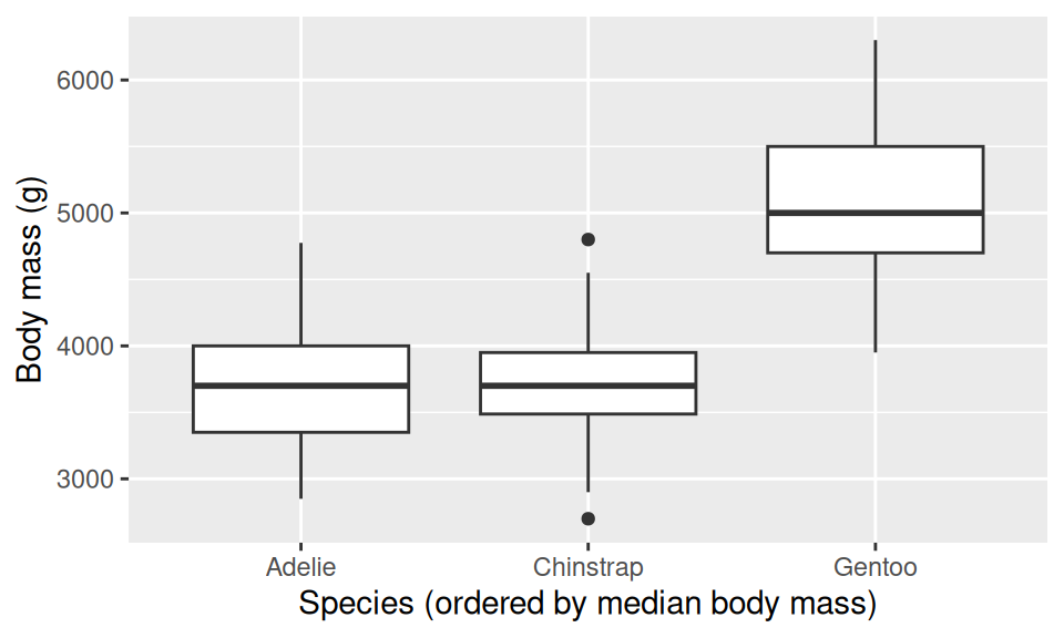

Without fct_reorder(), species appear alphabetically: Adelie, Chinstrap, Gentoo. With it, they appear in order of median body mass. This is where factors click: the plot labels reflect the data, not the alphabet.

Exercises

Use fct_infreq() on penguins$island to see which island has the most observations.
Use fct_lump_n() with n = 1 on penguins$species. What happens?
Create a bar chart of penguins$species with bars ordered by frequency (hint: fct_infreq() inside aes()).

12.6 Dates and times

Time zones, leap years, daylight saving, and varying month lengths make date arithmetic surprisingly tricky.

R has three date-time classes:

Date: date only, stored as days since 1970-01-01
POSIXct: date + time, stored as seconds since 1970-01-01 (compact, use in data frames)
POSIXlt: date + time as a named list of components (rarely needed)

today <- Sys.Date()
today
#> [1] "2026-03-09"
typeof(today)
#> [1] "double"
unclass(today)
#> [1] 20521

The number from unclass() is days since the Unix epoch. Dates in R count from 1970-01-01 because Unix measured time as seconds from that date. 32-bit signed integers can count seconds from 1970 until January 19, 2038 (the “Year 2038 problem”). R, Python, JavaScript, and most databases all inherit this epoch. Date arithmetic works:

as.Date("2026-03-07") - as.Date("2026-01-01")
#> Time difference of 65 days

R returns a difftime object. Dates understand addition and subtraction.

as.Date("2026-01-01") + 30
#> [1] "2026-01-31"

The base R parsing function is as.Date(). It expects ISO 8601 format ("YYYY-MM-DD") by default:

as.Date("2026-03-07")
#> [1] "2026-03-07"
as.Date("07/03/2026", format = "%d/%m/%Y")
#> [1] "2026-03-07"

The format argument uses %Y (4-digit year), %m (month), %d (day), and similar codes. These are hard to remember, which is why lubridate exists.

Exercises

What day number (since 1970-01-01) is today? Use unclass(Sys.Date()).
What date is 1000 days from today? Use Sys.Date() + 1000.
How many days are between "2024-02-28" and "2024-03-01"? (2024 is a leap year.)

12.7 lubridate: dates for humans

lubridate’s parsing functions are named after the order of components. The function name tells you the format:

ymd("2026-03-07")
#> [1] "2026-03-07"
dmy("07/03/2026")
#> [1] "2026-03-07"
mdy("03-07-2026")
#> [1] "2026-03-07"

All three produce the same date. No format strings, no %Y/%m/%d to remember. The function name is the format.

For date-times:

ymd_hms("2026-03-07 14:30:00")
#> [1] "2026-03-07 14:30:00 UTC"

Extracting components:

d <- ymd("2026-03-07")
year(d)
#> [1] 2026
month(d)
#> [1] 3
day(d)
#> [1] 7
wday(d, label = TRUE)
#> [1] Sat
#> Levels: Sun < Mon < Tue < Wed < Thu < Fri < Sat

Date arithmetic with human-readable units:

d + days(30)
#> [1] "2026-04-06"
d + months(1)
#> [1] "2026-04-07"
d + years(1)
#> [1] "2027-03-07"

lubridate handles month-length differences correctly. Adding one month to January 31 gives February 28 (or 29 in a leap year), not an error.

lubridate distinguishes three kinds of time spans:

Duration: exact number of seconds. ddays(1) is always 86400 seconds.
Period: human units. days(1) is “one day,” which could be 23 or 25 hours around daylight saving transitions.
Interval: an anchored span with a start and end.

For most work, periods (days(), months(), years()) are what you want. Durations (ddays(), dmonths()) matter when you need physical time.

# How old is R? (first public release: 1993-08-01)
interval(ymd("1993-08-01"), Sys.Date()) %/% years(1)
#> [1] 32

Opinion

Parse with lubridate, extract with lubridate, do arithmetic with lubridate. Touch base R date functions only if you have zero dependencies.

Exercises

Parse the following dates: "15-Jan-2024", "2024/06/30", "December 25, 2023". Which lubridate function does each need?
What day of the week were you born? Use ymd() and wday(label = TRUE).
Compute the number of days between "2020-03-01" and "2026-03-01". Then compute the number of months using interval() and %/%.

12.8 Summary

Each of these data types has a matching tidyverse package:

Data type	Base R	Tidyverse package	Prefix
Text	`paste()`, `grep()`, `sub()`	stringr	`str_`
Categories	`factor()`, `levels()`	forcats	`fct_`
Dates	`as.Date()`, `Sys.Date()`	lubridate	`ymd()`, `year()`, …

The tidyverse packages give these operations a consistent interface and naming scheme. In some cases (like str_detect vs grepl) it is mostly cosmetic; in others (like lubridate’s timezone handling) the package catches real bugs that base R silently lets through.

In Chapter 11, you learned to structure data. In this chapter, you learned to handle the three messiest column types. In Chapter 14, you will combine both: transforming and summarizing data frames with dplyr, using stringr, forcats, and lubridate inside mutate() and filter() calls.