5  Your first function

sqrt(9), c(1, 2, 3), sum(x > 70): every piece of R code so far has relied on functions that someone else wrote. This chapter shows you how to write your own.

5.1 Anatomy of a function

A function in R has three parts: a name, arguments, and a body.

double <- function(x) x * 2

function(x) declares one parameter called x. The body, x * 2, is the expression R evaluates when you call the function, and double is the name you are binding this function to (the same way x <- 3 binds a name to a number).

Call it:

double(5)
#> [1] 10

double(c(1, 2, 3))
#> [1] 2 4 6

The second call works because * is vectorized (Section 4.4): the body x * 2 already operates element by element, so double handles vectors without a loop, without any extra effort on your part. But what happens when the body grows beyond a single expression?

A function with a longer body uses curly braces:

describe <- function(x) {
  n <- length(x)
  m <- mean(x)
  paste("n =", n, ", mean =", round(m, 2))
}

describe(c(72, 85, 61, 90, 78))
#> [1] "n = 5 , mean = 77.2"

The body is a block of expressions that R evaluates in order, returning the value of the last one. This is the same rule from Section 3.3: a block in curly braces is itself an expression, and its value is whatever the final line produces.

Exercises

1. Write a function square that takes a number and returns its square.
2. Write a function to_celsius that converts a Fahrenheit temperature to Celsius (formula: (f - 32) * 5/9). Test it with to_celsius(212).
3. Does to_celsius(c(32, 72, 212)) work? Why?

5.2 Arguments and defaults

Functions can have multiple arguments, and some can have default values:

greet <- function(name, greeting = "Hello") {
  paste(greeting, name)
}

name is required; greeting is optional, defaulting to "Hello" if you leave it out:

greet("R")
#> [1] "Hello R"

greet("R", "Hey")
#> [1] "Hey R"

You can also pass arguments by name, in any order:

greet(greeting = "Bonjour", name = "R")
#> [1] "Bonjour R"

This is the same positional-versus-named distinction from Section 3.4, when we used log(8, base = 2). The rule is uniform across R because function calls all work the same way, whether you wrote the function or someone at R Core did.

Some functions accept a variable number of arguments using ... (pronounced “dot-dot-dot”):

shout <- function(...) {
  words <- c(...)
  toupper(paste(words, collapse = " "))
}

shout("hello", "world")
#> [1] "HELLO WORLD"

... collects every argument you pass, however many there are, and c(...) combines them into a vector. This is a surprisingly deep idea. In Church’s lambda calculus (Section 1.2), a function takes exactly one argument; if you want two, you write a function that returns another function:

λx. λy. x + y

This reads: “a function that takes x and returns another function that takes y and returns x + y.” To add 3 and 5, you apply it twice: (λx. λy. x + y)(3)(5) = (λy. 3 + y)(5) = 3 + 5 = 8. Each application replaces one argument, one step at a time. This is called currying, and R can do it too (Chapter 20). ... is R’s practical alternative: instead of nesting functions, you let a single function accept any number of arguments and decide what to do with them inside. c(), paste(), sum(): they all use ..., which is why c(1, 2, 3) and c(1, 2, 3, 4, 5, 6, 7) both work. More on ... in Chapter 23.

Exercises

1. Write a function power with arguments x and n = 2 that computes x^n. Test it with power(3) and power(3, 3).
2. What happens if you call greet() with no arguments? Read the error message.
3. Rewrite power so the default exponent is 3. What does power(2) return now?

5.3 Return values

R returns the value of the last expression in the body. No keyword needed:

add_one <- function(x) x + 1
add_one(10)
#> [1] 11

The body is x + 1. R evaluates it and returns the result. In Python or Java you would need to write return explicitly, but R treats the last expression as the return value. A function is an expression that evaluates to a value, the same idea from the lambda calculus in Section 2.1.

When you call add_one(10), R substitutes 10 for x in the body, turning x + 1 into 10 + 1, then evaluates it. Lambda calculus calls this beta reduction: (λx. x + 1)(10) reduces to 10 + 1. Every function call in R is a beta reduction.

R does have a return() function, and it is useful for early exits:

safe_log <- function(x) {
  if (any(x <= 0)) return(NA)
  log(x)
}

safe_log(5)
#> [1] 1.609438
safe_log(-1)
#> [1] NA

If x has any non-positive values, the function exits immediately and returns NA. Otherwise, it falls through to log(x).

TipOpinion

Use return() only for early exits like safe_log above. If the function runs to the end, let the last expression be the return value; writing return(x) on the last line adds nothing but noise.

One subtlety: assignment returns its value invisibly. When a function’s last line is an assignment, R returns the value but does not print it:

quiet <- function(x) {
  result <- x + 1
}

quiet(5)

Nothing printed. The function returned 6, but invisibly. If you want to see it:

(quiet(5))
#> [1] 6

Or store it:

y <- quiet(5)
y
#> [1] 6

The general rule: if you want your function to show a result, make sure the last expression is the value itself, not an assignment. But there is a deeper question lurking here: if a function is just a value, can you treat it the way you treat a number or a string?

Exercises

1. What does this function return? Predict, then check:

   mystery <- function(x) {
     a <- x + 1
     b <- a * 2
     b
   }
   mystery(3)

2. What about this one?

   mystery2 <- function(x) {
     a <- x + 1
     b <- a * 2
   }
   mystery2(3)

3. Write a function clamp that takes a value x, a lo, and a hi, and returns lo if x < lo, hi if x > hi, and x otherwise. Use return() for the early exits.

5.4 Functions are just values

Type sqrt without parentheses and R prints the function itself, not a result. A function is a value, the same kind of thing as a number or a string: you can assign it, put it in a list, or interrogate its type.

f <- double
f(5)
#> [1] 10

is.function(double)
#> [1] TRUE

typeof(double)
#> [1] "closure"

double is a name bound to a value, and that value happens to be a function. f <- double gives the same function a second name, which is exactly what happened in Section 3.2 when y <- x gave the number 3 a second name.

You can even create a function without giving it a name at all:

(function(x) x + 1)(10)
#> [1] 11

function(x) x + 1 creates a function; the parentheses around it and (10) immediately call it with the argument 10. This is an anonymous function: λx. x + 1 applied to 10 (Section 1.2). Chapter 19 uses them heavily.

You can do anything with a function that you can do with a number: store it in a variable, pass it to another function, return it as a result. This is what McCarthy built into Lisp in 1958 (Section 2.1), and R inherits it directly. So functions are values, and values live somewhere. Where do the variables inside a function live?

Exercises

1. Assign sqrt to a new name s. Does s(16) work?
2. What does is.function(42) return? What about is.function(is.function)?
3. Run (function(a, b) a + b)(3, 4). What happens?

5.5 Scope: a first look

What happens to variables created inside a function?

add_ten <- function(x) {
  y <- 10
  x + y
}

add_ten(5)
#> [1] 15

y was created inside add_ten. Can you access it from outside?

y
#> [1] 6

No. Variables created inside a function live in the function’s own local environment and vanish when the function finishes. This is what makes functions safe: they do not leak their internal state into your workspace. But the boundary is not symmetric.

multiplier <- 3

scale <- function(x) {
  x * multiplier
}

scale(10)
#> [1] 30

scale found multiplier in the workspace because it was not defined inside the function body. R looks for names first in the local environment, then in the environment where the function was defined, a strategy called lexical scoping that R inherited from Scheme (Section 2.2).

If a function can read outer variables, can it change them?

n <- 0

increment <- function() {
  n <- n + 1
  n
}

increment()
#> [1] 1
n
#> [1] 0

increment created its own local n, set it to 1, and returned it, but the n in the workspace is still 0. The function read the outer n without modifying it; it created a new local binding with the same name. This is R’s copy-on-modify philosophy: values do not change, you create new values.

The practical rule is simple: what happens inside a function stays inside the function. The full machinery behind this (environments, closures, and the scope chain) is in Chapter 18.

Exercises

1. Predict the output, then run it:

   x <- 100
   f <- function() {
     x <- 1
     x
   }
   f()
   x

2. What does this return?

   x <- 10
   g <- function(x) {
     x + 1
   }
   g(20)

   Is it 11 or 21? Why?

3. Can a function call another function you’ve defined? Try it: write triple <- function(x) x * 3, then write triple_and_add <- function(x) triple(x) + 1. Does triple_and_add(5) work?

5.6 Guarding your inputs

What happens when someone passes the wrong type to your function?

to_celsius <- function(f) (f - 32) * 5/9
to_celsius("hot")
#> Error in `f - 32`:
#> ! non-numeric argument to binary operator

The error says non-numeric argument to binary operator, which is technically accurate but unhelpful: you have to read the function body to figure out what went wrong. Better to catch the problem at the door:

to_celsius <- function(f) {
  stopifnot(is.numeric(f))
  (f - 32) * 5/9
}

to_celsius("hot")
#> Error in `to_celsius()`:
#> ! is.numeric(f) is not TRUE

stopifnot() checks a condition and stops with an error if it is FALSE. The message now tells you exactly what failed: is.numeric(f) is not TRUE. You can stack multiple checks in the same call:

safe_divide <- function(x, y) {
  stopifnot(is.numeric(x), is.numeric(y), y != 0)
  x / y
}

safe_divide(10, 0)
#> Error in `safe_divide()`:
#> ! y != 0 is not TRUE

A function that fails immediately with a clear message saves you from chasing wrong outputs later. Chapter 25 covers input validation in depth; for now, stopifnot() at the top of your functions is enough. But validation only protects against bad inputs. What about the structure of the computation itself?

Exercises

1. Add a stopifnot() to your power function that checks x is numeric and n is numeric.
2. What happens if you write stopifnot(is.numeric(x), length(x) == 1) and pass a vector? Try it.

5.7 Recursion

A function can call other functions. Can it call itself?

factorial <- function(n) {
  if (n == 0) return(1)
  n * factorial(n - 1)
}

factorial(5)
#> [1] 120

factorial(5) calls factorial(4), which calls factorial(3), and so on, until factorial(0) returns 1 and the whole chain collapses back:

factorial(5)
= 5 * factorial(4)
= 5 * 4 * factorial(3)
= 5 * 4 * 3 * factorial(2)
= 5 * 4 * 3 * 2 * factorial(1)
= 5 * 4 * 3 * 2 * 1 * factorial(0)
= 5 * 4 * 3 * 2 * 1 * 1
= 120

This is recursion: a function defined in terms of itself. Look at the unfolding carefully. Each line replaces a function call with its value, the same term replacement from Section 4.2, and no variable is being updated, no counter is ticking. The answer was implicit in the original expression factorial(5); evaluation simply made it explicit.

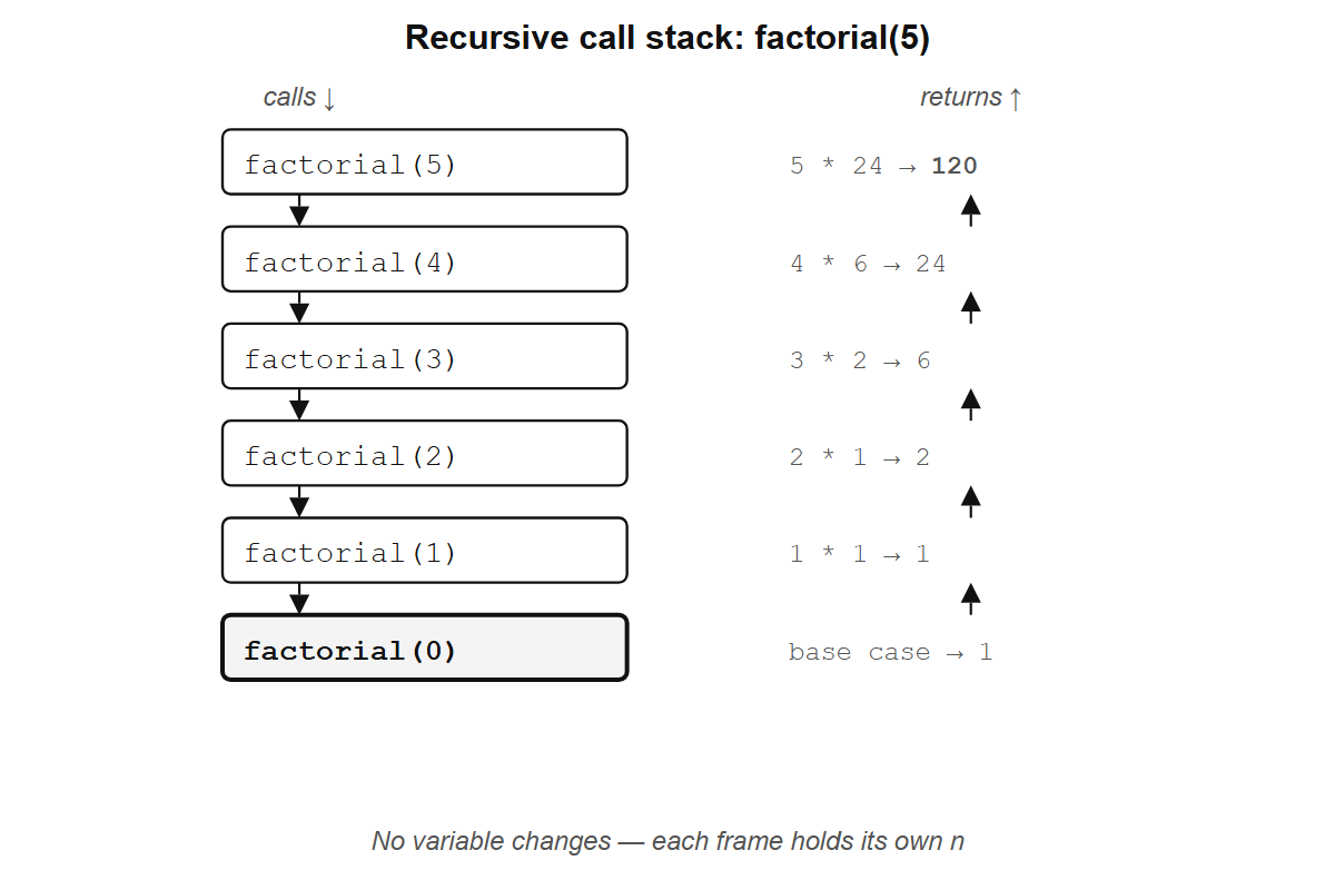
Figure 5.1: Recursive call stack for factorial(5): each frame waits for the one below it. No variable changes — each frame holds its own n.

In lambda calculus notation, factorial looks like this:

fact = λn. if n = 0 then 1 else n * fact(n - 1)

(This self-reference is informal shorthand; pure lambda calculus has no names, so fact cannot refer to itself directly. Section 30.5 shows how recursion works without them.)

Wait. In Section 1.2, the lambda calculus had only three things: variables, functions, and application. Where did if/then/else come from? Church showed that you can encode true, false, and conditional branching as pure lambda functions:

TRUE  = λx. λy. x      # a function that takes two arguments and returns the first
FALSE = λx. λy. y      # a function that takes two arguments and returns the second
IF    = λcond. λthen. λelse. cond(then)(else)

TRUE is a function that picks its first argument; FALSE picks its second. IF just hands both options to the condition and lets it choose. So IF(TRUE)(1)(2) becomes TRUE(1)(2) becomes (λx. λy. x)(1)(2) becomes 1. The entire conditional is built from functions choosing between arguments, and the if n = 0 then 1 else ... notation above is shorthand for this encoding.

The reduction works as before, one substitution at a time:

fact(3)                                     # apply fact with n = 3
= (λn. if n=0 then 1 else n * fact(n-1))(3) # replace fact with its definition
= if 3=0 then 1 else 3 * fact(3-1)          # substitute n = 3
= 3 * fact(2)                               # 3≠0, so take the else branch
= 3 * 2 * fact(1)                           # same pattern: n=2, substitute, reduce
= 3 * 2 * 1 * fact(0)                       # n=1
= 3 * 2 * 1 * 1                             # n=0, take the then branch: 1
= 6

R’s function(n) is the same as λn. The reduction above is what R does when you call factorial(3): substitute 3 for n, evaluate the body, hit factorial(2), substitute again, keep going until the base case. Recursion is how Church’s lambda calculus (Section 1.2) handles repetition. There is no loop counter; the function calls itself with a smaller argument until it stops.

fibonacci <- function(n) {
  if (n <= 1) return(n)
  fibonacci(n - 1) + fibonacci(n - 2)
}

fibonacci(10)
#> [1] 55

Recursion is elegant but not always practical. fibonacci(30) is already slow because it recomputes the same values over and over: fibonacci(10) calls fibonacci(9) and fibonacci(8), but fibonacci(9) also calls fibonacci(8), so that subtree gets computed twice. Further down, fibonacci(7) gets computed three times, fibonacci(6) five times, and the work grows exponentially. Is there a way to keep the recursive structure without paying the exponential cost?

A smarter version avoids this by carrying the last two values forward as arguments:

fibonacci_fast <- function(n, a = 0, b = 1) {
  if (n == 0) return(a)
  fibonacci_fast(n - 1, b, a + b)
}

fibonacci_fast(10)
#> [1] 55
fibonacci_fast(50)
#> [1] 12586269025

Instead of branching into two recursive calls, fibonacci_fast makes one call per step, passing the accumulated values along. Watch the reduction:

fibonacci_fast(4, 0, 1)
= fibonacci_fast(3, 1, 1)    # n=4→3, a=0→1, b=1→0+1=1
= fibonacci_fast(2, 1, 2)    # n=3→2, a=1→1, b=1→1+1=2
= fibonacci_fast(1, 2, 3)    # n=2→1, a=1→2, b=2→1+2=3
= fibonacci_fast(0, 3, 5)    # n=1→0, a=2→3, b=3→2+3=5
= 3                           # n=0, return a

No variable is being mutated; each call just substitutes new values for n, a, and b and hands them to the next call. This form is called tail recursion because the recursive call is the last thing the function does. The naive version cannot compute fibonacci(50) in any reasonable time. This one handles it instantly:

Any function with multiple recursive calls can be rewritten as a single recursive call with extra arguments that carry the intermediate results. For Fibonacci, the state to pass forward is the last two numbers; for a tree traversal, it might be an accumulator list.

R has a limit on how deep recursion can go (around 1000 calls by default), and for most day-to-day R work, vectorized operations and functions like map() (Chapter 19) are better tools. But there is something strange about factorial that has nothing to do with performance: its base case and inductive step look exactly like a proof by mathematical induction.

Exercises

1. Trace through factorial(3) by hand, writing out each step like the example above.
2. Write a recursive function sum_to that adds up all integers from 1 to n. Check: sum_to(100) should return 5050.
3. What happens if you call factorial(-1)? Why? Add a stopifnot() to guard against it.

5.8 Programs and proofs

Look at factorial again:

factorial <- function(n) {
  if (n == 0) return(1)
  n * factorial(n - 1)
}

Two parts: a base case (when n = 0, return 1) and an inductive step (assume factorial(n - 1) gives the right answer, and use it to compute factorial(n)). If you have seen mathematical induction, you recognize the shape immediately. A proof by induction has a base case and an inductive step too. The resemblance is not a coincidence.

In the 1930s and 1940s, the logician Haskell Curry (after whom the Haskell programming language is named, and from whom the term “currying” above comes) noticed something strange: the rules for combining types in a programming language looked identical to the rules for combining propositions in formal logic. A function that takes an A and returns a B had the same structure as a logical proof that “if A, then B.” In 1969, William Howard made this precise: every type corresponds to a logical proposition, and every program of that type corresponds to a proof of that proposition. A recursive function that terminates is a proof by induction. This result is called the Curry-Howard correspondence.

Writing factorial constructs a proof by induction that the product 1 * 2 * ... * n exists for every non-negative integer. The transformation from double-recursive fibonacci to tail-recursive fibonacci_fast is the same move a logician makes when they strengthen an inductive hypothesis to make a proof go through: the extra arguments (a and b) are the stronger hypothesis. Double induction reduces to simple induction with stronger invariants, which is why the same trick turns a slow recursive function into a fast one.

This was the landscape of the 1930s: Church, Godel, Curry, and Turing were all studying what could be proved, before computers existed, and they found that the answer was identical to what could be computed.

Today, the Curry-Howard correspondence is the foundation of formal verification: software that proves other software is correct.

The first practical tool to exploit this idea was Coq, developed at INRIA, the French national computer science institute, starting in the late 1980s. Thierry Coquand and Gerard Huet designed it around a type theory called the Calculus of Constructions (the “C-o-C” that gives Coq part of its name). In Coq, every program must come with a machine-checkable proof that it does what its type signature claims; if the proof has a gap, the code does not compile. This makes Coq painful for ordinary programming but powerful for building software where correctness matters more than convenience.

In 2013, Leonardo de Moura at Microsoft Research started Lean, a newer proof assistant with a more accessible syntax and a growing library of formalized mathematics called Mathlib. Coq grew out of theoretical computer science; Lean has attracted a broader community of mathematicians who are formalizing results from analysis, algebra, and number theory. In Lean, a proof that adding zero to any natural number gives back the same number looks like this:

theorem add_zero (n : Nat) : n + 0 = n := by
  induction n with
  | zero => rfl
  | succ n ih => simp [Nat.add_succ, ih]

The structure is identical to factorial: a base case (zero), an inductive step (succ n), and the result from the smaller case (ih, the induction hypothesis). If the proof is wrong, the code does not compile. The proof is a program, and the program is a proof.

The definition of factorial says that factorial(n) and n * factorial(n - 1) are the same expression for arbitrary n, an equivalence that holds by term replacement alone, without evaluating either side. It is true by definition. The base case says factorial(0) is 1, also by definition. Those two statements are the entire proof: you show that the program in state n and the program in state n - 1 are the same program up to one substitution, and that the chain has a starting point. That is a proof by induction, and it covers every natural number at once. In lambda calculus notation:

fact = λn. if n = 0 then 1 else n * fact(n - 1)

fact is the function. fact(n) is the function applied to some n. Replacing the name fact with its definition gives:

fact(n)
= (λn. if n = 0 then 1 else n * fact(n - 1))(n)   # replace fact with its definition
= if n = 0 then 1 else n * fact(n - 1)              # substitute n

You might think: of course they are the same, we just wrote the definition. But fact and fact(n) are not the same thing. fact is a definition, a rule that says what to do with an argument; fact(n) is that rule applied to a specific (but arbitrary) n. The reduction above shows what happens when you apply the rule: you get a term that contains fact(n - 1), the same program applied to a smaller argument. That relationship between fact(n) and fact(n - 1) is not something we assumed or proved; it fell out of one substitution. A tautology. And yet that tautology, together with the base case, constitutes a proof by induction that fact produces the right answer for every natural number. When n = 0, the expression reduces to 1. The substitution gives you the step from n - 1 to n.

This is what Curry-Howard means in practice. The Lean proof above has the same structure as factorial: a base case (zero), a step that relates n to n - 1 by definitional equivalence (succ n), and nothing else. Both work because the equivalence of two program states is a tautology that requires only substitution.

The seL4 microkernel (used in military helicopters and autonomous vehicles) has a machine-checked proof that certain classes of errors in its code cannot occur, for any input. Not “we haven’t found a bug yet”: a mathematical guarantee, verified by a computer. The CompCert C compiler has a similar proof that it will never miscompile your code. Both proofs were written as programs in Coq. Traditional testing covers a finite set of inputs; a proof by induction, because it operates on the structure of the program rather than on specific values, covers all of them.

R does not enforce this connection the way Coq or Lean do. But the structure is there underneath, in every recursive function you write, with its base case and its inductive step, carrying the same shape as a proof that holds for all natural numbers. You have been writing proofs this whole chapter. You just did not need to call them that.