Extract posterior distributions of temporally-varying coefficients (TVCs) from a fitted ratio model with TVC specification.
Usage
tvc(
  object,
  terms = NULL,
  group = 1L,
  summary = FALSE,
  probs = c(0.025, 0.5, 0.975),
  ...
)

# S3 method for class 'ratiod_fit'
tvc(
  object,
  terms = NULL,
  group = 1L,
  summary = FALSE,
  probs = c(0.025, 0.5, 0.975),
  ...
)

# S3 method for class 'ratiod_tvc_posterior'
print(x, ...)

# S3 method for class 'ratiod_tvc_posterior'
summary(object, probs = c(0.025, 0.5, 0.975), ...)

# S3 method for class 'ratiod_tvc_posterior'
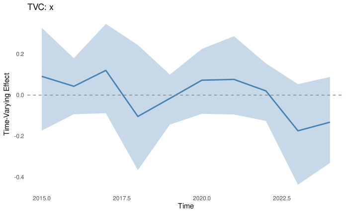
plot(x, term = 1, type = "ribbon", ...)
Arguments
- object
A
ratiod_fitobject fitted withtvcargument- terms
Which TVC terms to extract. If NULL (default), extracts all.
- group
Which level of the temporal grouping variable to report, as an index into its levels; a model without temporal groups has the one level 1.
- summary
Logical; if TRUE, return summary statistics instead of full posterior draws.
- probs
Quantiles to compute if
summary = TRUE.- ...
Ignored
- x
A ratiod_tvc_posterior object
- term
Which term to plot (name or index). Default: first term.
- type
Plot type: "ribbon" (default) or "line"
Value
A ratiod_tvc_posterior object containing:
draws: Array of posterior draws (draws x times x terms)time_levels: Time point labelsterm_names: Names of TVC terms
See also
temporal_tvc(), plot.ratiod_tvc_posterior()
Examples
# \donttest{
# Generate synthetic data
set.seed(160)
df <- data.frame(
year = rep(2015:2024, each = 5),
x = rnorm(50),
count = rpois(50, lambda = 18),
effort = rgamma(50, shape = 3.5, rate = 1)
)
# Fit model with TVC
fit <- tratio(
count | effort ~ x,
data = df,
family = ratiod_poisson_gamma(),
temporal = temporal_tvc("year", terms = c(1, 2)),
mode = "hmc",
control = list(iter = 400, chains = 1, seed = 1)
)
# Extract TVC posteriors
tvc_post <- tvc(fit)
summary(tvc_post)
#> time_idx time term mean sd q2.5 q50
#> 1 1 2015 (Intercept) -0.081871821 0.09212934 -0.255463018 -0.092316519
#> 2 2 2016 (Intercept) -0.087068939 0.08564337 -0.287968373 -0.085775005
#> 3 3 2017 (Intercept) -0.158440935 0.11448729 -0.352905848 -0.159007504
#> 4 4 2018 (Intercept) -0.057286795 0.09555183 -0.271986762 -0.061236841
#> 5 5 2019 (Intercept) 0.043315616 0.08132142 -0.110746254 0.045453422
#> 6 6 2020 (Intercept) 0.015838640 0.08265069 -0.136829010 0.022217114
#> 7 7 2021 (Intercept) 0.001094192 0.10841945 -0.216776562 0.003272936
#> 8 8 2022 (Intercept) 0.072019887 0.07866050 -0.110137172 0.073642983
#> 9 9 2023 (Intercept) 0.227137901 0.10516914 0.002057857 0.225636852
#> 10 10 2024 (Intercept) 0.024702365 0.09737968 -0.160441604 0.023010991
#> 11 1 2015 x 0.091404548 0.13984520 -0.172407870 0.095695649
#> 12 2 2016 x 0.043056580 0.07358915 -0.093177191 0.045334524
#> 13 3 2017 x 0.120645339 0.12426567 -0.088133698 0.119087628
#> 14 4 2018 x -0.103886408 0.16706493 -0.365530666 -0.108735637
#> 15 5 2019 x -0.015931552 0.06234091 -0.143596189 -0.019244288
#> 16 6 2020 x 0.072801637 0.08249411 -0.091017228 0.067688847
#> 17 7 2021 x 0.076703856 0.10816594 -0.094501335 0.071803152
#> 18 8 2022 x 0.020605535 0.07239532 -0.125847074 0.016525183
#> 19 9 2023 x -0.173756099 0.13816865 -0.436512214 -0.153878372
#> 20 10 2024 x -0.131801687 0.11685598 -0.330681967 -0.143844856
#> q97.5
#> 1 0.09070951
#> 2 0.09223756
#> 3 0.06532319
#> 4 0.13067963
#> 5 0.20016965
#> 6 0.15030765
#> 7 0.21039655
#> 8 0.21923672
#> 9 0.44399389
#> 10 0.19965029
#> 11 0.32774011
#> 12 0.17996041
#> 13 0.34721392
#> 14 0.24436137
#> 15 0.10027463
#> 16 0.22514230
#> 17 0.28723674
#> 18 0.15454488
#> 19 0.05356365
#> 20 0.08863310
# Plot temporal evolution
plot(tvc_post, "x")
 # }
# }