• tulpaRatio

title: “Spatial and Temporal Models” author: “Gilles Colling” date: “2026-08-04” output: rmarkdown::html_vignette vignette: > % % %

Overview

This vignette covers spatial and temporal extensions in numdenom. These allow borrowing strength across neighboring locations or time points, improving estimates in data-sparse regions.

Spatial Models

numdenom supports two spatial priors for areal (discrete region) data:

Function	Prior	Use Case
`spatial_car()`	Intrinsic CAR (ICAR)	Simple spatial smoothing
`spatial_bym2()`	BYM2	Interpretable spatial fraction

Both require an adjacency matrix defining which regions are neighbors.

Creating Adjacency Matrices

From Coordinates (Grid Data)

# Camera trap grid
n <- 25
coords <- expand.grid(x = 1:5, y = 1:5)

# Queen contiguity (8 neighbors)
adj <- matrix(0, n, n)
for (i in 1:n) {
  for (j in 1:n) {
    if (i != j) {
      dist <- sqrt((coords$x[i] - coords$x[j])^2 +
                   (coords$y[i] - coords$y[j])^2)
      if (dist <= sqrt(2) + 0.01) adj[i, j] <- 1
    }
  }
}

From sf Objects

library(sf)
library(spdep)

# From shapefile
regions <- st_read("regions.shp")
nb <- poly2nb(regions, queen = TRUE)
adj <- nb2mat(nb, style = "B", zero.policy = TRUE)

ICAR Model: `spatial_car()`

The intrinsic conditional autoregressive (ICAR) prior encourages neighboring regions to have similar effects:

$\phi_i | \phi_{-i} \sim \text{Normal}\left(\frac{1}{n_i}\sum_{j \sim i} \phi_j, \frac{\sigma^2}{n_i}\right)$

where $j \sim i$ denotes neighbors of region $i$ .

fit <- tratio(
  count | effort ~ x + (1 | region),
  spatial = spatial_car(
    adj = adj,
    level = "group",
    group_var = "region"
  ),
  data = df,
  family = ratiod_poisson_gamma()
)

Parameters

adj: Square binary adjacency matrix
level: "group" (one effect per group) or "obs" (one per observation)
group_var: Variable name matching the grouping factor (required if level = "group")

BYM2 Model: `spatial_bym2()`

The BYM2 reparameterization (Riebler et al., 2016) separates spatial structure from unstructured heterogeneity:

$\theta_i = \sigma \left(\sqrt{\rho} \cdot \phi_i^* + \sqrt{1-\rho} \cdot v_i\right)$

where: - $\phi_i^*$ is the scaled ICAR component - $v_i \sim \text{Normal}(0, 1)$ is unstructured noise - $\rho \in [0, 1]$ is the proportion of variance that is spatial

fit <- tratio(
  cases | population ~ age + (1 | county),
  spatial = spatial_bym2(
    adj = adj,
    level = "group",
    group_var = "county"
  ),
  data = df,
  family = ratiod_binomial()
)

The $\rho$ parameter is directly interpretable: $\rho = 0.8$ means 80% of the random effect variance is spatially structured.

Extracting Spatial Effects

# Get posterior summaries
spatial_effects <- extract_spatial(fit)

# Map visualization
library(ggplot2)
library(sf)

regions$spatial_effect <- spatial_effects$mean
ggplot(regions) +
geom_sf(aes(fill = spatial_effect)) +
  scale_fill_gradient2()

Temporal Models

numdenom supports temporal priors for time series structure:

Function	Prior	Use Case
`temporal_rw()`	Random walk	Smooth trends
`temporal_ar1()`	AR(1)	Mean-reverting dynamics

Random Walk: `temporal_rw()`

First-order random walk (RW1):

$\gamma_t | \gamma_{t-1} \sim \text{Normal}(\gamma_{t-1}, \sigma_\gamma^2)$

Second-order random walk (RW2) for smoother trends:

$\gamma_t | \gamma_{t-1}, \gamma_{t-2} \sim \text{Normal}(2\gamma_{t-1} - \gamma_{t-2}, \sigma_\gamma^2)$

# First-order random walk
fit <- tratio(
  count | effort ~ x + (1 | site),
  temporal = temporal_rw(
    time_var = "year",
    order = 1
  ),
  data = df,
  family = ratiod_poisson_gamma()
)

# Second-order for smoother trends
fit <- tratio(
  count | effort ~ x,
  temporal = temporal_rw(
    time_var = "year",
    order = 2
  ),
  data = df,
  family = ratiod_poisson_gamma()
)

Cyclic Random Walk

For seasonal patterns that wrap around (e.g., month 12 neighbors month 1):

fit <- tratio(
  count | effort ~ x,
  temporal = temporal_rw(
    time_var = "month",
    order = 1,
    cyclic = TRUE
  ),
  data = df,
  family = ratiod_poisson_gamma()
)

AR(1): `temporal_ar1()`

Autoregressive order 1:

$\gamma_t = \rho \cdot \gamma_{t-1} + \epsilon_t, \quad \epsilon_t \sim \text{Normal}(0, \sigma_\gamma^2)$

The correlation parameter $\rho \in (-1, 1)$ controls persistence.

fit <- tratio(
  count | effort ~ x,
  temporal = temporal_ar1(
    time_var = "year"
  ),
  data = df,
  family = ratiod_poisson_gamma()
)

Group-Specific Temporal Effects

By default, temporal effects are shared across all groups. For group-specific trends:

fit <- tratio(
  count | effort ~ (1 | site),
  temporal = temporal_rw(
    time_var = "year",
    group_var = "site",
    shared = FALSE
  ),
  data = df,
  family = ratiod_poisson_gamma()
)

Extracting Temporal Effects

# Year-level effects
temporal_effects <- extract_temporal(fit)

# Plot trend
library(ggplot2)
ggplot(temporal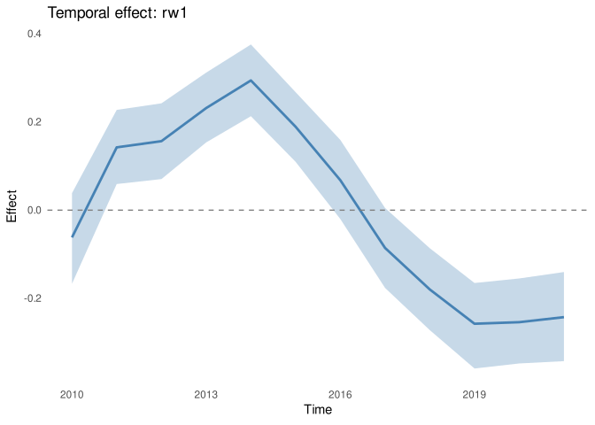_effects, aes(x = year, y = mean)) +
  geom_ribbon(aes(ymin = q2.5, ymax = q97.5), alpha = 0.2) +
  geom_line() +
  labs(y = "Temporal effect")

Combining Spatial and Temporal

For spatiotemporal data, include both:

fit <- tratio(
  count | effort ~ x + (1 | region),
  spatial = spatial_bym2(adj, level = "group", group_var = "region"),
  temporal = temporal_rw(time_var = "year"),
  data = df,
  family = ratiod_poisson_gamma()
)

This fits additive spatial and temporal effects. For interaction effects, see the next section.

Spatiotemporal Interaction

When spatial patterns change over time (or temporal trends differ across space), additive models may be insufficient. numdenom supports spatiotemporal interaction effects following Knorr-Held (2000).

Interaction Types

Type	Description	Parameters
Type I	Unstructured (IID)	$S \times T$
Type II	Structured time at each location	$S \times T$
Type III	Structured space at each time	$S \times T$
Type IV	Fully structured (Kronecker)	$S \times T$
Separable	For GP spatial/temporal	$S \times T$

Type I: Unstructured Interaction

The simplest form assumes independent random effects for each space-time combination:

$\delta_{st} \stackrel{iid}{\sim} \text{Normal}(0, \sigma_\delta^2)$

fit <- tratio(
  count | effort ~ x,
  data = df,
  family = ratiod_poisson_gamma(),
  spatiotemporal = spatiotemporal(
    spatial = spatial_car(adj, level = "group", group_var = "region"),
    temporal = temporal_rw1("year"),
    type = "I"
  )
)

Type II: Structured Time at Each Location

Each location has its own temporal random walk:

$\delta_{\cdot t}^{(s)} \sim \text{RW}(\sigma^2)$

This captures location-specific temporal trends.

fit <- tratio(
  count | effort ~ x,
  data = df,
  family = ratiod_poisson_gamma(),
  spatiotemporal = spatiotemporal(
    spatial = spatial_car(adj, level = "group", group_var = "region"),
    temporal = temporal_rw1("year"),
    type = "II"
  )
)

Type III: Structured Space at Each Time Point

Each time point has its own spatial field:

$\delta_{s \cdot}^{(t)} \sim \text{ICAR}(\tau)$

This captures time-specific spatial patterns.

fit <- tratio(
  count | effort ~ x,
  data = df,
  family = ratiod_poisson_gamma(),
  spatiotemporal = spatiotemporal(
    spatial = spatial_car(adj, level = "group", group_var = "region"),
    temporal = temporal_rw1("year"),
    type = "III"
  )
)

Type IV: Fully Structured (Kronecker)

Precision is the Kronecker product of spatial and temporal precision:

$Q_\delta = Q_s \otimes Q_t$

This is the most constrained and often most appropriate model.

fit <- tratio(
  count | effort ~ x,
  data = df,
  family = ratiod_poisson_gamma(),
  spatiotemporal = spatiotemporal(
    spatial = spatial_car(adj, level = "group", group_var = "region"),
    temporal = temporal_rw1("year"),
    type = "IV"
  )
)

Non-Separable Spatiotemporal GP

For continuous space-time data, use spatiotemporal_gp() with non-separable covariance:

fit <- tratio(
  count | effort ~ x,
  data = df,
  family = ratiod_poisson_gamma(),
  spatiotemporal = spatiotemporal_gp(
    ~ lon + lat,
    time_var = "date",
    nonsep_type = "gneiting"
  )
)

Non-separability types:

"product": Separable (reference)
"sum": Additive covariance
"gneiting": Gneiting (2002) class
"cressie_huang": Cressie-Huang (1999) class

Extracting Spatiotemporal Effects

# Summary format
st_effects <- spatiotemporal_effects(fit, format = "summary")
head(st_effects)

# Array format (S x T x draws)
st_array <- spatiotemporal_effects(fit, format = "array")

# Visualization
plot(st_effects, type = "heatmap")
plot(st_effects, type = "time_series")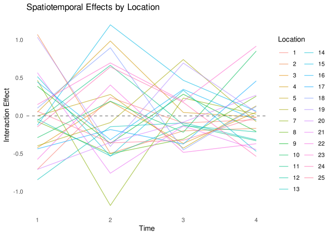

Model Selection

Compare interaction types using LOO-CV:

fit_type1 <- tratio(..., spatiotemporal = spatiotemporal(..., type = "I"))
fit_type4 <- tratio(..., spatiotemporal = spatiotemporal(..., type = "IV"))

loo_compare(loo(fit_type1), loo(fit_type4))

Prior Specification

Spatial Priors

fit <- tratio(
  ...,
  spatial = spatial_car(adj, level = "group", group_var = "region"),
  priors = ratiod_priors(
    tau_spatial_shape = 1.0,  # Gamma shape for precision
    tau_spatial_rate = 0.01   # Gamma rate for precision
  )
)

Temporal Priors

fit <- tratio(
  ...,
  temporal = temporal_rw(time_var = "year"),
  priors = ratiod_priors(
    tau_temporal_shape = 2.0,
    tau_temporal_rate = 0.5
  )
)