Quick Start

Installation

pak::pak("gcol33/tulpaRatio")

library(tulpaRatio)

What tulpaRatio Does

tulpaRatio fits Bayesian hierarchical models for ratios, rates, and proportions. Instead of modelling ratios directly (which is statistically problematic), tulpaRatio jointly models the numerator and denominator processes, then derives ratios with full uncertainty propagation.

See vignette("philosophy") for the statistical motivation.

The Three Families

tulpaRatio provides three model families for common ratio types:

Family	Numerator	Denominator	Use Case
`ratiod_negbin_negbin()`	Counts	Counts	Relative abundance, species ratios
`ratiod_binomial()`	Successes	Trials	Detection rates, survival
`ratiod_poisson_gamma()`	Counts	Continuous	CPUE, catch per effort

Basic Example: CPUE Analysis

Catch per unit effort with site-level variation:

# Simulated trawl data
set.seed(123)
n_sites <- 20
n_obs <- 200

trawl_data <- data.frame(
  site = factor(rep(1:n_sites, each = n_obs/n_sites)),
  depth = rnorm(n_obs),  # standardised depth
  season = factor(sample(c("spring", "summer", "fall"), n_obs, replace = TRUE)),
  weather = factor(sample(c("calm", "rough"), n_obs, replace = TRUE))
)
# A site effect raises both effort and catch; catch per unit effort
# falls with depth
site_effect <- rnorm(n_sites, 0, 0.4)[trawl_data$site]
trawl_data$effort <- rgamma(n_obs, shape = 5, rate = 5 / exp(1 + site_effect))
trawl_data$catch <- rpois(n_obs, trawl_data$effort *
                            exp(1 + site_effect - 0.3 * trawl_data$depth))

# Fit model
fit <- tratio(
  catch | effort ~ depth + season + (1 | site),
  data = trawl_data,
  family = ratiod_poisson_gamma(),
  control = list(seed = 1)
)

# View results
summary(fit)
#> ratio model summary
#> ===================
#> 
#> Inference: Exact (Tier 1) via hmc
#> Family: poisson_gamma 
#> 
#> Fixed effects (numerator):
#>         parameter   mean    sd   2.5%  97.5%  rhat ess_bulk
#>   num:(Intercept)  2.180 0.141  1.910  2.450 1.021      209
#>         num:depth -0.321 0.025 -0.371 -0.272 1.000     1602
#>  num:seasonspring  0.112 0.058 -0.003  0.225 1.004     1079
#>  num:seasonsummer -0.067 0.055 -0.174  0.043 1.002      878
#> 
#> Fixed effects (denominator):
#>           parameter   mean    sd   2.5% 97.5%  rhat ess_bulk
#>   denom:(Intercept)  1.104 0.146  0.829 1.395 1.021      206
#>         denom:depth -0.022 0.035 -0.092 0.051 1.007     1356
#>  denom:seasonspring -0.013 0.085 -0.176 0.155 1.003     1029
#>  denom:seasonsummer -0.092 0.078 -0.244 0.058 1.003      999
#> 
#> Variance components:
#>  parameter  mean    sd  2.5% 97.5%  rhat ess_bulk
#>      shape 5.078 0.537 4.103 6.196 1.002     1630
#>   sigma_re 0.593 0.111 0.423 0.847 1.014      237
#> 
#> Diagnostics:
#>   Divergences: 0 
#>   Avg. acceptance: 0.899 
#>   Chains: 4 
#>   Iterations: 2000 
#>   Warmup: 1000 
#>   R-hat > 1.01 for 3 parameter(s), largest 1.021 (num:(Intercept)).
#>   Bulk ESS < 400 for 3 parameter(s), smallest 206 (denom:(Intercept)).
#>   Run longer chains or reparameterise before using these estimates.

Extract CPUE Posteriors

# Observation-level CPUE
cpue <- ratio(fit)
summary(cpue)
#> tulpaRatio ratio summary (response scale)
#> ===========================================
#> 
#>  obs     mean        sd     q2.5      q50    q97.5
#>    1 3.476484 0.2458432 3.004140 3.471393 3.973538
#>    2 3.149342 0.2124233 2.745451 3.145960 3.572252
#>    3 1.850111 0.1724552 1.532138 1.844759 2.203628
#>    4 3.266236 0.2493155 2.803865 3.255744 3.778108
#>    5 3.209494 0.2459214 2.749787 3.199425 3.709867
#>    6 1.766526 0.1728818 1.446776 1.759545 2.119285
#>    7 2.627668 0.1885765 2.277621 2.619202 3.018554
#>    8 4.295104 0.3655295 3.596578 4.282692 5.027857
#>    9 3.701099 0.2599391 3.217723 3.691493 4.247946
#>   10 3.810627 0.2941414 3.260944 3.794842 4.409698
#> 
#> ... and 190 more rows

# Compare CPUE between seasons
ratio_contrast(fit, ~ season)
#> tulpaRatio ratio contrasts
#> =====================
#> 
#> Type: difference 
#> Variable: season 
#> Reference: fall 
#> 
#>        contrast       mean         sd        q2.5        q50     q97.5
#>  spring vs fall 0.15651737 0.10204919 -0.04705321 0.15564659 0.3522177
#>  summer vs fall 0.06264186 0.09088572 -0.11212026 0.06123507 0.2454185
#>  prob_positive
#>         0.9375
#>         0.7530

Formula Syntax

Combined Formula (Recommended)

Use num | denom ~ predictors when both processes share predictors:

fit <- tratio(
  catch | effort ~ depth + season + (1 | site),
  data = trawl_data,
  family = ratiod_poisson_gamma(),
  control = list(seed = 1)
)

Process-Specific Predictors

Add terms that affect only numerator or denominator:

fit_split <- tratio(
  catch | effort ~ (1 | site),           # Shared structure
  formula_num = ~ depth + season,         # Catch-specific

  formula_denom = ~ weather,              # Effort-specific
  data = trawl_data,
  family = ratiod_poisson_gamma(),
  control = list(seed = 1)
)
coef(fit_split)
#>    num:(Intercept)          num:depth   num:seasonspring   num:seasonsummer 
#>         2.18399756        -0.32133756         0.11018633        -0.06673448 
#>  denom:(Intercept) denom:weatherrough 
#>         1.10204001        -0.06044949

Random Effects

The examples in this section use simulated counts y out of totals n, with a covariate x, plots nested in sites, and survey years crossed with sites:

set.seed(42)
counts <- expand.grid(plot = 1:3, site = 1:12, year = 1:10)
site_eff <- rnorm(12, 0, 0.4)
year_eff <- rnorm(10, 0, 0.3)
plot_eff <- rnorm(36, 0, 0.2)
slope_eff <- rnorm(12, 0, 0.2)
eta <- site_eff[counts$site] + year_eff[counts$year] +
  plot_eff[(counts$site - 1) * 3 + counts$plot]
counts$x <- rnorm(nrow(counts))
counts$n <- rnbinom(nrow(counts), size = 10, mu = 60 * exp(eta))
counts$y <- rnbinom(nrow(counts), size = 10,
                    mu = 12 * exp(eta + (0.3 + slope_eff[counts$site]) * counts$x))
counts[c("plot", "site", "year")] <- lapply(counts[c("plot", "site", "year")], factor)
ctrl <- list(seed = 1)

Random Intercepts

# Single grouping factor
fit_re <- tratio(y | n ~ x + (1 | site), data = counts, control = ctrl)

# Multiple (crossed) grouping factors
fit_re <- tratio(y | n ~ x + (1 | site) + (1 | year), data = counts, control = ctrl)

# Nested grouping factors
fit_re <- tratio(y | n ~ x + (1 | site/plot), data = counts, control = ctrl)

Random Slopes

# Correlated intercept and slope
fit_re <- tratio(y | n ~ x + (1 + x | site), data = counts, control = ctrl)

# Uncorrelated (independent) intercept and slope
fit_re <- tratio(y | n ~ x + (1 + x || site), data = counts, control = ctrl)

Model Checking

# Posterior predictive checks
pp_check(fit, type = "dens_overlay")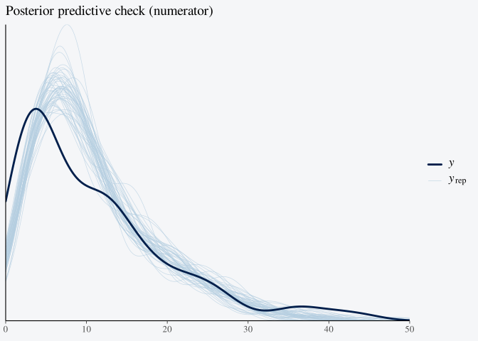


# Model comparison
loo(fit)
#> Warning: Some Pareto k diagnostic values are too high. See help('pareto-k-diagnostic') for details.
#> 
#> Computed from 4000 by 200 log-likelihood matrix.
#> 
#>          Estimate   SE
#> elpd_loo  -1014.3 43.4
#> p_loo        70.7  9.4
#> looic      2028.6 86.9
#> ------
#> MCSE of elpd_loo is NA.
#> MCSE and ESS estimates assume independent draws (r_eff=1).
#> 
#> Pareto k diagnostic values:
#>                          Count Pct.    Min. ESS
#> (-Inf, 0.7]   (good)     197   98.5%   205     
#>    (0.7, 1]   (bad)        3    1.5%   <NA>    
#>    (1, Inf)   (very bad)   0    0.0%   <NA>    
#> See help('pareto-k-diagnostic') for details.
waic(fit)
#> Warning: 
#> 45 (22.5%) p_waic estimates greater than 0.4. We recommend trying loo instead.
#> 
#> Computed from 4000 by 200 log-likelihood matrix.
#> 
#>           Estimate   SE
#> elpd_waic  -1013.0 43.2
#> p_waic        69.4  9.1
#> waic        2026.0 86.4
#> 
#> 45 (22.5%) p_waic estimates greater than 0.4. We recommend trying loo instead.

# Compare models
fit1 <- tratio(catch | effort ~ depth + (1 | site), data = trawl_data,
               family = ratiod_poisson_gamma(), control = ctrl)
fit2 <- tratio(catch | effort ~ depth + season + (1 | site), data = trawl_data,
               family = ratiod_poisson_gamma(), control = ctrl)
ratiod_compare(fit1, fit2)
#> Warning: Some Pareto k diagnostic values are too high. See help('pareto-k-diagnostic') for details.
#>  model elpd_diff se_diff p_worse       diag_diff      diag_elpd
#>   fit1       0.0     0.0      NA                               
#>   fit2      -0.7     7.1    0.54 |elpd_diff| < 4 3 k_psis > 0.7
#> 
#> Diagnostic flags present.
#> See ?`loo-glossary` (sections `diag_diff` and `diag_elpd`)
#> or https://mc-stan.org/loo/reference/loo-glossary.html.

The |elpd_diff| < 4 flag marks a difference too small to separate the two models: adding season does not improve the expected predictive accuracy.

Both criteria print warnings here. Each site effect is estimated from ten observations, so leaving one observation out moves it noticeably: waic() then reports observations whose p_waic exceeds 0.4 and recommends loo(), and loo() flags the observations whose Pareto $k$ is too high for importance sampling to follow. Their contributions to elpd_loo are less reliable than the rest, which the standard errors do not show.

Quick Reference

Function	Purpose
`tratio()`	Fit model
`ratio()`	Extract ratio posteriors
`ratio_contrast()`	Compare ratios between groups
`pp_check()`	Posterior predictive checks
`loo()`, `waic()`	Model comparison
`ratiod_compare()`	Compare multiple models

Gilles Colling

2026-10-13