Installation
install.packages("pak")                   # development version
pak::pak("gcol33/tulpaRatio")
Overview
This vignette demonstrates complete analysis workflows using
tulpaRatio. Each example shows data preparation, model fitting,
diagnostics, and inference. See vignette("getting-started")
for basic usage and vignette("philosophy") for statistical
motivation.
Workflow 1: Fisheries CPUE
Goal: Estimate standardized catch per unit effort (CPUE) while accounting for varying effort and site effects.
Challenge: Effort varies systematically across sites and seasons. Sites with more effort appear to have more precise CPUE, but this precision is illusory if effort correlates with catch conditions.
Strategy: Joint model with shared site effects.
Data
library(tulpaRatio)

# Simulated fisheries data
set.seed(42)
n_sites <- 15
n_seasons <- 4
n_obs <- n_sites * n_seasons * 3

fisheries <- data.frame(
  site = factor(rep(1:n_sites, each = n_seasons * 3)),
  season = factor(rep(rep(c("spring", "summer", "fall", "winter"), each = 3), n_sites)),
  depth = rnorm(n_obs, 50, 20),
  catch = rpois(n_obs, lambda = 20),
  effort_hours = rgamma(n_obs, shape = 4, rate = 0.5)
)

head(fisheries)
#>   site season    depth catch effort_hours
#> 1    1 spring 77.41917    20     3.777342
#> 2    1 spring 38.70604    17     5.003239
#> 3    1 spring 57.26257    20    13.266320
#> 4    1 summer 62.65725    26     8.140340
#> 5    1 summer 58.08537    17     8.155921
#> 6    1 summer 47.87751    23     2.735758
Model Fitting
fit_cpue <- tratio(
  catch | effort_hours ~ depth + season + (1 | site),
  data = fisheries,
  family = ratiod_poisson_gamma(),
  control = list(seed = 1)
)

summary(fit_cpue)
#> ratio model summary
#> ===================
#>
#> Inference: Exact (Tier 1) via hmc
#> Family: poisson_gamma
#>
#> Fixed effects (numerator):
#>         parameter   mean    sd   2.5% 97.5%  rhat ess_bulk
#>   num:(Intercept)  2.998 0.055  2.894 3.105 1.002     1192
#>         num:depth  0.000 0.001 -0.002 0.002 1.002     2305
#>  num:seasonspring -0.041 0.046 -0.130 0.051 1.003     1059
#>  num:seasonsummer  0.000 0.048 -0.096 0.094 1.003     1128
#>  num:seasonwinter -0.022 0.048 -0.121 0.073 1.004     1107
#>
#> Fixed effects (denominator):
#>           parameter   mean    sd   2.5% 97.5%  rhat ess_bulk
#>   denom:(Intercept)  2.008 0.138  1.737 2.276 1.006     1201
#>         denom:depth  0.000 0.002 -0.004 0.005 1.004     2467
#>  denom:seasonspring  0.058 0.121 -0.176 0.291 1.005     1021
#>  denom:seasonsummer  0.126 0.121 -0.109 0.365 1.002     1141
#>  denom:seasonwinter -0.085 0.121 -0.322 0.152 1.004     1072
#>
#> Variance components:
#>  parameter  mean    sd  2.5% 97.5%  rhat ess_bulk
#>      shape 3.123 0.310 2.549 3.754 1.001     2083
#>   sigma_re 0.041 0.024 0.003 0.092 1.002      675
#>
#> Diagnostics:
#>   Divergences: 0
#>   Avg. acceptance: 0.941
#>   Chains: 4
#>   Iterations: 2000
#>   Warmup: 1000
Diagnostics
# Check convergence
plot(fit_cpue, type = "trace")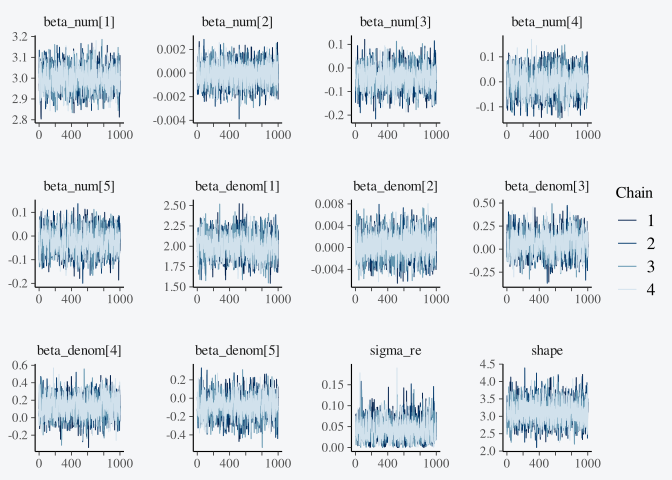
# Posterior predictive checks
pp_check(fit_cpue, type = "dens_overlay", component = "numerator")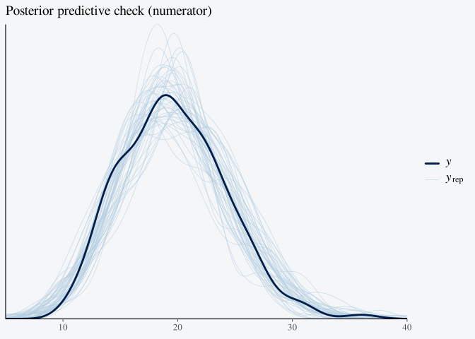
pp_check(fit_cpue, type = "dens_overlay", component = "denominator")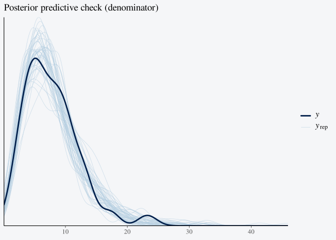
Inference
# Site-level CPUE estimates
cpue_by_site <- ratio(fit_cpue, by = "site")
summary(cpue_by_site)
#> tulpaRatio ratio summary (response scale)
#> ===========================================
#>
#>  group     mean        sd     q2.5      q50    q97.5
#>      1 2.501800 0.1515746 2.216152 2.498036 2.802372
#>      2 2.534810 0.1292860 2.286392 2.530990 2.795708
#>      3 2.520943 0.1168142 2.300605 2.519017 2.751370
#>      4 2.530357 0.1225129 2.293190 2.527843 2.776059
#>      5 2.519244 0.1173015 2.295996 2.518228 2.750099
#>      6 2.511110 0.1267746 2.270314 2.508759 2.757399
#>      7 2.518622 0.1176070 2.295603 2.518159 2.750836
#>      8 2.516321 0.1193380 2.290457 2.514558 2.750853
#>      9 2.519861 0.1170661 2.297092 2.517956 2.750286
#>     10 2.523908 0.1171424 2.304013 2.521994 2.759336
#>
#> ... and 5 more rows

# Seasonal contrasts
ratio_contrast(fit_cpue, ~ season)
#> tulpaRatio ratio contrasts
#> =====================
#>
#> Type: difference
#> Variable: season
#> Reference: fall
#>
#>        contrast        mean        sd       q2.5         q50     q97.5
#>  spring vs fall -0.09771824 0.1269284 -0.3456825 -0.09654990 0.1448983
#>  summer vs fall -0.12684419 0.1291322 -0.3821485 -0.12476850 0.1218282
#>  winter vs fall  0.06254843 0.1293123 -0.1934804  0.06144407 0.3202047
#>  prob_positive
#>          0.219
#>          0.162
#>          0.695

# Effect of depth
predict(
  fit_cpue,
  newdata = data.frame(depth = c(30, 50, 70), season = "summer"),
  re_formula = NA
)
#> tulpaRatio predictions
#> =================
#>
#> Posterior draws: 4000
#> New observations: 3
#>
#>  obs component     mean        sd     q2.5      q50    q97.5
#>    1     ratio 2.349730 0.2473360 1.894748 2.336845 2.877198
#>    2     ratio 2.321842 0.2137299 1.918366 2.313329 2.756052
#>    3     ratio 2.299450 0.2345963 1.845495 2.290074 2.782424
Workflow 2: Relative Abundance
Goal: Estimate the proportion of a target species relative to total catch across habitats.
Challenge: Both target count and total count are overdispersed. Using binomial models would underestimate uncertainty.
Strategy: Negative binomial for both counts with shared observer effects.
Data
set.seed(123)
n_plots <- 30
n_visits <- 4

abundance <- data.frame(
  plot = factor(rep(1:n_plots, each = n_visits)),
  habitat = factor(rep(sample(c("forest", "grassland", "wetland"), n_plots, replace = TRUE), each = n_visits)),
  observer = factor(sample(1:10, n_plots * n_visits, replace = TRUE))
)

# Plot and observer effects scale target and total counts alike; the
# target share is higher in grassland and lower in wetland
u <- rnorm(n_plots, sd = 0.4)[abundance$plot] + rnorm(10, sd = 0.4)[abundance$observer]
hab <- c(forest = 0, grassland = 0.4, wetland = -0.3)[as.character(abundance$habitat)]
abundance$target_count <- rnbinom(n_plots * n_visits, size = 3, mu = 15 * exp(u + hab))
abundance$total_count <- rnbinom(n_plots * n_visits, size = 5, mu = 50 * exp(u))

# Ensure target <= total
abundance$target_count <- pmin(abundance$target_count, abundance$total_count)
Model
fit_abundance <- tratio(
  target_count | total_count ~ habitat + (1 | plot) + (1 | observer),
  data = abundance,
  family = ratiod_negbin_negbin(),
  control = list(seed = 1)
)

summary(fit_abundance)
#> ratio model summary
#> ===================
#>
#> Inference: Exact (Tier 1) via hmc
#> Family: negbin_negbin
#>
#> Fixed effects (numerator):
#>             parameter   mean    sd   2.5% 97.5%  rhat ess_bulk
#>       num:(Intercept)  2.443 0.296  1.861 3.017 1.011      371
#>  num:habitatgrassland  0.589 0.234  0.136 1.055 1.016      539
#>    num:habitatwetland -0.197 0.249 -0.682 0.283 1.010      489
#>
#> Fixed effects (denominator):
#>               parameter  mean    sd   2.5% 97.5%  rhat ess_bulk
#>       denom:(Intercept) 3.617 0.291  3.023 4.190 1.011      358
#>  denom:habitatgrassland 0.230 0.214 -0.174 0.653 1.018      474
#>    denom:habitatwetland 0.283 0.222 -0.157 0.707 1.011      443
#>
#> Variance components:
#>    parameter  mean    sd  2.5% 97.5%  rhat ess_bulk
#>    phi_denom 4.974 0.797 3.565 6.711 1.003     1639
#>      phi_num 3.053 0.544 2.136 4.265 1.001     2105
#>  sigma_re[1] 0.382 0.071 0.262 0.545 1.003      686
#>  sigma_re[2] 0.688 0.228 0.401 1.215 1.008      420
#>
#> Diagnostics:
#>   Divergences: 0
#>   Avg. acceptance: 0.893
#>   Chains: 4
#>   Iterations: 2000
#>   Warmup: 1000
#>   R-hat > 1.01 for 6 parameter(s), largest 1.018 (denom:habitatgrassland).
#>   Bulk ESS < 400 for 2 parameter(s), smallest 358 (denom:(Intercept)).
#>   Run longer chains or reparameterise before using these estimates.
Results
# Habitat effects on relative abundance
ratio_contrast(fit_abundance, ~ habitat)
#> tulpaRatio ratio contrasts
#> =====================
#>
#> Type: difference
#> Variable: habitat
#> Reference: forest
#>
#>             contrast       mean        sd        q2.5        q50      q97.5
#>  grassland vs forest  0.3586336 0.1926348 -0.03591693  0.3594662  0.7287145
#>    wetland vs forest -0.4807423 0.1963220 -0.88402404 -0.4786503 -0.1081355
#>  prob_positive
#>         0.9635
#>         0.0050

# Plot-level estimates
abundance_by_plot <- ratio(fit_abundance, by = "plot")
summary(abundance_by_plot)
#> tulpaRatio ratio summary (response scale)
#> ===========================================
#>
#>  group      mean         sd      q2.5       q50     q97.5
#>      1 0.1926232 0.02441532 0.1483814 0.1911210 0.2465666
#>      2 0.1926232 0.02441532 0.1483814 0.1911210 0.2465666
#>      3 0.1926232 0.02441532 0.1483814 0.1911210 0.2465666
#>      4 0.4457209 0.05515564 0.3492737 0.4417393 0.5658741
#>      5 0.1926232 0.02441532 0.1483814 0.1911210 0.2465666
#>      6 0.4457209 0.05515564 0.3492737 0.4417393 0.5658741
#>      7 0.4457209 0.05515564 0.3492737 0.4417393 0.5658741
#>      8 0.4457209 0.05515564 0.3492737 0.4417393 0.5658741
#>      9 0.1926232 0.02441532 0.1483814 0.1911210 0.2465666
#>     10 0.3125050 0.04713153 0.2338838 0.3080292 0.4171301
#>
#> ... and 20 more rows
Workflow 3: Detection Probability
Goal: Estimate detection probability from camera trap data with spatial structure.
Challenge: Detection varies by site characteristics and has spatial autocorrelation.
Strategy: Binomial model with spatial random effects.
Data
set.seed(456)
n_cameras <- 40

# Camera locations on a grid
coords <- expand.grid(x = 1:8, y = 1:5)
coords <- coords[1:n_cameras, ]

# Create adjacency matrix (queen contiguity)
adj <- matrix(0, n_cameras, n_cameras)
for (i in 1:n_cameras) {
  for (j in 1:n_cameras) {
    if (i != j) {
      dist <- sqrt((coords$x[i] - coords$x[j])^2 + (coords$y[i] - coords$y[j])^2)
      if (dist <= sqrt(2) + 0.01) adj[i, j] <- 1
    }
  }
}

camera_data <- data.frame(
  camera = factor(1:n_cameras),
  vegetation = rnorm(n_cameras),
  nights_active = sample(20:30, n_cameras, replace = TRUE)
)

# Detection varies smoothly across the grid
field <- 0.6 * sin(coords$x / 2) - 0.4 * cos(coords$y / 2)
camera_data$detections <- rbinom(
  n_cameras,
  size = camera_data$nights_active,
  prob = plogis(-0.8 + 0.3 * camera_data$vegetation + field)
)
Spatial Model
fit_detection <- tratio(
  detections | nights_active ~ vegetation,
  spatial = spatial_car(adj, level = "group", group_var = "camera"),
  data = camera_data,
  family = ratiod_binomial(),
  mode = "hmc",
  control = list(seed = 1)
)

summary(fit_detection)
#> ratio model summary
#> ===================
#>
#> Inference: Exact (Tier 1) via hmc
#> Family: binomial_fixed
#>
#> Fixed effects (numerator):
#>        parameter   mean    sd   2.5%  97.5%  rhat ess_bulk
#>  num:(Intercept) -0.535 0.071 -0.678 -0.396 1.002     2374
#>   num:vegetation  0.362 0.081  0.200  0.525 1.003     1644
#>
#> Variance components:
#>    parameter  mean    sd  2.5% 97.5%  rhat ess_bulk
#>  tau_spatial 2.575 1.983 0.785 6.952 1.009      327
#>
#> Diagnostics:
#>   Divergences: 0
#>   Avg. acceptance: 0.896
#>   Chains: 4
#>   Iterations: 2000
#>   Warmup: 1000
#>   Bulk ESS < 400 for 1 parameter(s), smallest 327 (tau_spatial).
#>   Run longer chains or reparameterise before using these estimates.
Spatial Predictions
# Camera-level detection probabilities
detection_probs <- ratio(fit_detection, by = "camera", summary = TRUE)
detection_probs
#> tulpaRatio ratio summary (response scale)
#> ===========================================
#>
#>  group      mean         sd      q2.5       q50     q97.5
#>      1 0.2747639 0.07233564 0.1449086 0.2705005 0.4262028
#>      2 0.4936835 0.07493091 0.3499779 0.4913731 0.6481016
#>      3 0.4673041 0.07435340 0.3247962 0.4655575 0.6145831
#>      4 0.2171653 0.05573067 0.1182847 0.2153865 0.3360561
#>      5 0.2695972 0.06100245 0.1642022 0.2668273 0.4050315
#>      6 0.2428791 0.05833906 0.1382330 0.2412561 0.3606778
#>      7 0.3340325 0.06328623 0.2168918 0.3302386 0.4609020
#>      8 0.2174379 0.06435022 0.1037323 0.2147610 0.3505500
#>      9 0.5345036 0.06914163 0.3987513 0.5338705 0.6671925
#>     10 0.4541477 0.06323844 0.3333352 0.4527835 0.5766218
#>
#> ... and 30 more rows

# Visualize spatial pattern
plot_map(as.data.frame(detection_probs), coords = coords)
Workflow 4: Temporal Trends
Goal: Estimate annual trends in population indices while accounting for temporal autocorrelation.
Strategy: Random walk prior on year effects.
Model with Temporal Structure
A temporal effect shared by numerator and denominator cancels in
their ratio, so the walk on the index uses shared = FALSE;
the warning this prints notes that such a walk can also absorb
unmeasured year-to-year drivers of the ratio.
fit_trend <- tratio(
  count | effort ~ (1 | site),
  temporal = temporal_rw1(time_var = "year", shared = FALSE),
  data = trend_data,
  family = ratiod_poisson_gamma(),
  control = list(seed = 1)
)
#> Warning: Non-shared temporal effects (shared = FALSE) may lead to confounded ratio estimates.
#> Consider whether temporal effects should be shared between
#> numerator and denominator to prevent spurious temporal patterns in ratios.

summary(fit_trend)
#> ratio model summary
#> ===================
#>
#> Inference: Exact (Tier 1) via hmc
#> Family: poisson_gamma
#>
#> Fixed effects (numerator):
#>        parameter mean    sd  2.5% 97.5% rhat ess_bulk
#>  num:(Intercept) 2.97 0.056 2.857 3.085 1.01      347
#>
#> Fixed effects (denominator):
#>          parameter  mean    sd  2.5% 97.5%  rhat ess_bulk
#>  denom:(Intercept) 1.551 0.067 1.418 1.685 1.009      395
#>
#> Variance components:
#>     parameter   mean     sd  2.5%  97.5%  rhat ess_bulk
#>         shape  4.609  0.518 3.656  5.681 1.001     1883
#>      sigma_re  0.160  0.054 0.086  0.287 1.004      598
#>  tau_temporal 24.084 11.604 8.601 52.474 1.004     1267
#>
#> Other parameters:
#>     parameter   mean    sd   2.5%  97.5%  rhat ess_bulk
#>   temporal[1] -0.155 0.071 -0.294 -0.020 1.005     2506
#>  temporal[10]  0.107 0.061 -0.011  0.221 1.001     2772
#>  temporal[11] -0.327 0.072 -0.469 -0.190 1.001     2430
#>  temporal[12] -0.293 0.071 -0.429 -0.153 1.003     2411
#>  temporal[13] -0.280 0.070 -0.415 -0.141 1.004     2550
#>  temporal[14] -0.389 0.074 -0.531 -0.250 1.001     2201
#>  temporal[15] -0.194 0.074 -0.343 -0.053 1.001     2604
#>   temporal[2]  0.129 0.059  0.011  0.244 1.000     2793
#>   temporal[3]  0.185 0.060  0.068  0.300 1.001     2485
#>   temporal[4]  0.309 0.055  0.200  0.414 1.002     3085
#>   temporal[5]  0.213 0.059  0.090  0.326 1.000     2722
#>   temporal[6]  0.454 0.056  0.343  0.563 1.001     2501
#>   temporal[7]  0.038 0.063 -0.085  0.161 1.001     2482
#>   temporal[8]  0.062 0.059 -0.056  0.171 1.003     2859
#>   temporal[9]  0.142 0.062  0.018  0.262 1.001     2768
#>
#> Diagnostics:
#>   Divergences: 0
#>   Avg. acceptance: 0.879
#>   Chains: 4
#>   Iterations: 2000
#>   Warmup: 1000
#>   R-hat > 1.01 for 1 parameter(s), largest 1.010 (num:(Intercept)).
#>   Bulk ESS < 400 for 2 parameter(s), smallest 347 (num:(Intercept)).
#>   Run longer chains or reparameterise before using these estimates.
Extract Trend
# Year-level index
trend_by_year <- ratio(fit_trend, by = "year")
summary(trend_by_year)
#> tulpaRatio ratio summary (response scale)
#> ===========================================
#>
#>  group     mean        sd     q2.5      q50    q97.5
#>      1 3.551171 0.2996972 3.005336 3.540741 4.176412
#>      2 4.712996 0.3305064 4.091140 4.705037 5.389153
#>      3 4.986130 0.3610972 4.315926 4.968533 5.738029
#>      4 5.638551 0.3767063 4.924234 5.633021 6.392492
#>      5 5.125771 0.3697842 4.422982 5.113821 5.892777
#>      6 6.518851 0.4475199 5.691346 6.504071 7.437888
#>      7 4.303034 0.3252749 3.682301 4.287694 4.946833
#>      8 4.409142 0.3140337 3.797058 4.410101 5.046036
#>      9 4.776843 0.3543760 4.106582 4.766975 5.483993
#>     10 4.610259 0.3355579 3.983959 4.593621 5.310866
#>
#> ... and 5 more rows

# Plot trend with uncertainty
plot(temporal(fit_trend))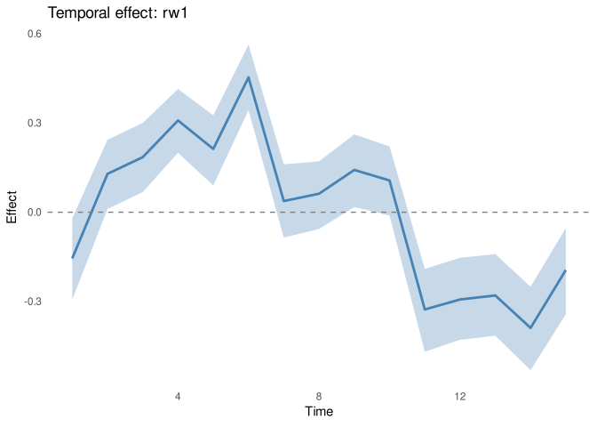
Summary
| Workflow | Family | Key Feature |
|---|---|---|
| Fisheries CPUE | poisson_gamma |
Shared site effects |
| Relative Abundance | negbin_negbin |
Overdispersed counts |
| Detection Probability | binomial |
Spatial CAR |
| Temporal Trends | poisson_gamma |
Random walk |
See Also
-
vignette("getting-started")- Basic usage -
vignette("philosophy")- Statistical motivation -
vignette("spatial-temporal")- Spatial and temporal details