Temporally Varying Coefficients (TVC)

Specify temporally-varying coefficients for ratio models. TVCs allow regression coefficients to change smoothly over time using a Gaussian process or random walk prior. This captures how effects evolve temporally.

Usage

temporal_tvc(
  time_var,
  terms = 1,
  structure = c("rw1", "rw2", "ar1", "iid", "gp"),
  group_var = NULL,
  shared = TRUE
)

# S3 method for class 'ratiod_tvc'
print(x, ...)

Arguments

time_var

Name of the time variable in data. Can be a formula (e.g., ~ year) or a character string (e.g., "year").

terms

Which coefficients should vary over time. Options:

Integer vector: Column indices of design matrix (1 = intercept)
Character vector: Coefficient names (e.g., "(Intercept)", "depth")
Formula: ~ 1 + depth for intercept and depth

structure

Temporal structure for the varying coefficients:

"rw1": First-order random walk (default)
"rw2": Second-order random walk (smoother)
"ar1": First-order autoregressive
"iid": Independent draws at each time point (no temporal smoothing)
"gp": Gaussian process (for irregular time spacing). Not yet implemented; temporal_tvc() errors if selected.

group_var

Optional name of grouping variable for panel data.

shared

Logical; if TRUE (default), TVC effects enter both numerator and denominator. Set to FALSE for process-specific TVCs (triggers warning about potential confounding).

x

A ratiod_tvc object

...

Ignored

Value

A ratiod_tvc object

Details

The TVC model extends the linear predictor:

$$\eta(t) = X\beta + \tilde{X}(t)w(t)$$

where:

$\beta$ are global (non-time-varying) coefficients
$\tilde{X}(t)$ is the subset of covariates with TVCs
$w(t)$ are time-varying adjustments

Each TVC follows a temporal process: $$w_j(t) \sim RW1(\sigma_j^2) \text{ or other temporal structure}$$

Interpretation: A positive TVC for depth at time t means the depth effect is stronger at t than the global average. The temporal variance $\sigma^2_j$ quantifies how much the effect varies over time.

Identifiability: TVCs are centered (sum-to-zero constraint) to separate the time-varying component from the global effect.

Examples

# Create TVC specification
tvc <- temporal_tvc("year", terms = 1)
print(tvc)
#> tulpaRatio temporally-varying coefficients
#> ======================================
#> 
#> Time variable: year 
#> Structure: RW1 (first-order random walk) 
#> Shared: Yes (enters both processes) 
#> 
#> Terms: columns  1 

# \donttest{
# Generate synthetic data with time-varying effect
set.seed(150)
df <- data.frame(
  year = rep(2010:2025, each = 5),
  x = rnorm(80),
  count = rpois(80, lambda = 20),
  effort = rgamma(80, shape = 4, rate = 1)
)

# Time-varying intercept (random temporal field)
fit <- tratio(
  count | effort ~ x,
  data = df,
  family = ratiod_poisson_gamma(),
  temporal = temporal_tvc("year", terms = 1),
  mode = "hmc",
  control = list(iter = 400, chains = 1, seed = 1)
)
summary(fit)
#> ratio model summary
#> ===================
#> 
#> Inference: Exact (Tier 1) via hmc
#> Family: poisson_gamma 
#> 
#> Fixed effects (numerator):
#>        parameter   mean    sd   2.5% 97.5%  rhat ess_bulk
#>  num:(Intercept)  3.008 0.026  2.959 3.057 1.022      132
#>            num:x -0.007 0.026 -0.055 0.047 1.036       85
#> 
#> Fixed effects (denominator):
#>          parameter   mean    sd  2.5% 97.5%  rhat ess_bulk
#>  denom:(Intercept)  1.343 0.042  1.26 1.435 1.014      166
#>            denom:x -0.028 0.045 -0.12 0.053 1.000      129
#> 
#> Variance components:
#>             parameter   mean    sd  2.5%  97.5%  rhat ess_bulk
#>                 shape  5.616 0.842 4.239  7.800 0.997      135
#>  tau_tvc[(Intercept)] 15.469 4.772 7.398 23.873 1.033       98
#> 
#> Other parameters:
#>             parameter   mean    sd   2.5% 97.5%  rhat ess_bulk
#>  tvc[(Intercept),t10] -0.018 0.070 -0.157 0.102 1.001      124
#>  tvc[(Intercept),t11] -0.009 0.081 -0.146 0.141 1.024       50
#>  tvc[(Intercept),t12]  0.057 0.080 -0.092 0.204 1.048       41
#>  tvc[(Intercept),t13]  0.016 0.076 -0.131 0.137 0.996       97
#>  tvc[(Intercept),t14] -0.059 0.081 -0.215 0.076 1.119       75
#>  tvc[(Intercept),t15] -0.002 0.080 -0.149 0.145 1.001      133
#>  tvc[(Intercept),t16] -0.034 0.086 -0.204 0.132 1.006       84
#>   tvc[(Intercept),t1] -0.025 0.096 -0.207 0.167 1.006       52
#>   tvc[(Intercept),t2]  0.081 0.080 -0.077 0.254 0.996      123
#>   tvc[(Intercept),t3] -0.010 0.077 -0.152 0.154 0.999       49
#>   tvc[(Intercept),t4] -0.134 0.085 -0.293 0.033 1.000       60
#>   tvc[(Intercept),t5]  0.030 0.082 -0.136 0.208 1.011      102
#>   tvc[(Intercept),t6]  0.055 0.072 -0.107 0.175 1.001       62
#>   tvc[(Intercept),t7]  0.153 0.071  0.012 0.289 1.006      174
#>   tvc[(Intercept),t8] -0.003 0.071 -0.151 0.118 1.022       86
#>   tvc[(Intercept),t9] -0.098 0.080 -0.272 0.048 0.998       57
#> 
#> Diagnostics:
#>   Divergences: 0 
#>   Avg. acceptance: 0.949 
#>   Chains: 1 
#>   Iterations: 400 
#>   Warmup: 200 
#>   R-hat > 1.01 for 9 parameter(s), largest 1.119 (tvc[(Intercept),t14]).
#>   Bulk ESS < 100 for 13 parameter(s), smallest 41 (tvc[(Intercept),t12]).
#>   Run longer chains or reparameterise before using these estimates.

# Time-varying effect of x
fit2 <- tratio(
  count | effort ~ x,
  data = df,
  family = ratiod_poisson_gamma(),
  temporal = temporal_tvc("year", terms = c("(Intercept)", "x"), structure = "rw2"),
  mode = "hmc",
  control = list(iter = 400, chains = 1, seed = 1)
)

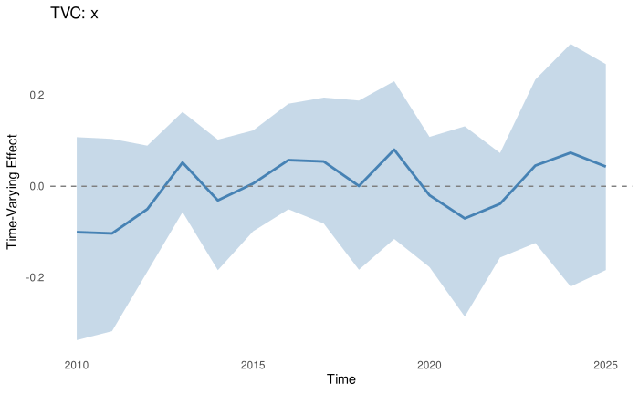
# Extract and plot the time-varying coefficients
tvc_effects <- tvc(fit2)
plot(tvc_effects, "x")

# }

Usage

Arguments

Value

Details

See also

Examples