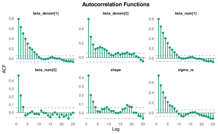
Creates autocorrelation function (ACF) plots for selected parameters. High autocorrelation indicates slow mixing and low effective sample size.
Details
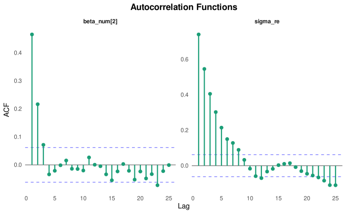
Ideal ACF plots show rapid decay to zero. Slow decay indicates high autocorrelation, which reduces effective sample size and may indicate poor mixing.
Examples
# \donttest{
sim <- sim_ratiod(n = 100, family = ratiod_poisson_gamma(), seed = 1)
fit <- tratio(y_num | y_denom ~ x1 + (1 | group), data = sim$data,
family = ratiod_poisson_gamma(),
control = list(iter = 1000, chains = 2, seed = 1))
plot_acf(fit)
 plot_acf(fit, pars = c("beta_num[2]", "sigma_re"))
 # }
# }