Multi-Scale Temporal Structure

Specify a multi-scale temporal random effect that decomposes temporal variation into trend, seasonal, and short-term components. Each component has its own variance parameter and structure.

This is particularly useful for long time series where patterns exist at multiple temporal scales (e.g., annual cycles, decadal trends).

Usage

temporal_multiscale(
  time_var,
  trend = c("rw2", "rw1", "none"),
  seasonal = NULL,
  short_term = c("ar1", "iid", "none"),
  group_var = NULL,
  shared = TRUE,
  parameterization = c("centered", "noncentered")
)

# S3 method for class 'ratiod_temporal_multiscale'
print(x, ...)

Arguments

time_var

Name of the time variable in data. Can be a formula (e.g., ~ year) or a character string (e.g., "year").

trend

Type of trend component: "rw2" (default, smooth), "rw1" (less smooth), or "none".

seasonal

Period for seasonal component (integer). Set to NULL or 0 for no seasonal component. Common values: 12 (monthly), 52 (weekly).

short_term

Type of short-term residual component: "ar1" (default, correlated), "iid" (independent), or "none".

group_var

Optional name of grouping variable for panel data.

shared

Logical; if TRUE (default), temporal effects enter both numerator and denominator.

parameterization

Coordinate the intrinsic trend and seasonal arms are sampled in. "centered" (default) samples the effects themselves. "noncentered" samples z ~ N(0, I) and reaches the effects through sigma * A^-1 z, where A stacks the arm's difference operator on 1'/sqrt(n), so the variance enters the linear predictor through the transform rather than through a quadratic form. The two describe the same model; what differs is the geometry the sampler sees. Prefer "noncentered" when an arm's variance is shrunk toward zero, where a centred coordinate leaves a funnel it cannot descend: on a 500-observation fixture whose true trend is zero, the divergence count goes 30 of 2000 to 3, the bulk ESS of sigma2_trend 21 to 310 and its rhat 1.13 to 1.01, and the centred run reports a posterior median four times larger because it never reaches the small end. The short-term arm is proper and is the same block either way.

x

A ratiod_temporal_multiscale object

...

Ignored

Value

A ratiod_temporal_multiscale object

Details

The multi-scale temporal model decomposes variation additively:

$$\eta(t) = trend(t) + seasonal(t) + short(t)$$

where:

• trend(t): Long-term smooth change via RW1 or RW2

• seasonal(t): Repeating pattern with period P via cyclic RW1

• short(t): Residual temporal correlation via AR(1) or IID

Each component has a separate variance parameter with PC priors to favor simpler models (fewer active components).

Sum-to-zero constraints are applied to trend and seasonal components for identifiability with the intercept.

See also

temporal_rw1(), temporal_rw2(), temporal_ar1() for single-component temporal effects, spatial_multiscale() for multi-scale spatial effects

Examples

# Create multi-scale temporal specification
temporal_multiscale("month_id", trend = "rw2", seasonal = 12, short_term = "ar1")
#> tulpaRatio Multi-Scale temporal specification
#> =========================================
#> 
#> Time variable: month_id 
#> 
#> Components:
#>   Trend: RW2 (second-order random walk, smooth) 
#>   Seasonal: Period = 12 (cyclic RW1)
#>   Short-term: AR(1) (autocorrelated residuals) 
#> 
#> Shared: Yes (enters both processes) 
temporal_multiscale("year", trend = "rw2", seasonal = NULL, short_term = "none")
#> tulpaRatio Multi-Scale temporal specification
#> =========================================
#> 
#> Time variable: year 
#> 
#> Components:
#>   Trend: RW2 (second-order random walk, smooth) 
#> 
#> Shared: Yes (enters both processes) 

# \donttest{
# Decompose into trend + seasonal + short-term
set.seed(129)
month_id <- 1:48
# Trend, 12-month cycle and AR(1) noise, shared by count and effort
eff <- 0.4 * sin(month_id / 15) + 0.4 * sin(2 * pi * month_id / 12) +
  as.numeric(arima.sim(list(ar = 0.6), 48, sd = 0.15))
x <- rnorm(48)
df <- data.frame(
  month_id = month_id,
  x = x,
  count = rpois(48, exp(3 + 0.3 * x + eff)),
  effort = rgamma(48, shape = 4, rate = exp(-eff))
)

fit <- tratio(
  count | effort ~ x,
  data = df,
  family = ratiod_poisson_gamma(),
  temporal = temporal_multiscale(
    time_var = "month_id",
    trend = "rw2",
    seasonal = 12,
    short_term = "ar1"
  ),
  control = list(iter = 1000, chains = 1, seed = 1)
)
#> Warning: 2 divergent transition(s) after warmup; raise `adapt_delta` or reparameterise.

# Extract and plot components
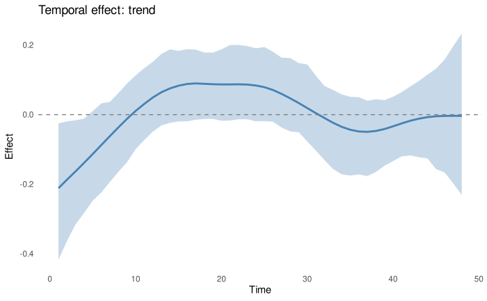
temporal_effects <- temporal(fit)
plot(temporal_effects, component = "trend")

# }