Zero-Inflation and Hurdle Models
Gilles Colling
2026-10-13
Source:vignettes/zero-inflation.Rmd
zero-inflation.RmdInstallation
install.packages("pak")                   # development version
pak::pak("gcol33/tulpaRatio")
Overview
Ecological and survey data often exhibit excess zeros beyond what standard distributions predict. tulpaRatio provides several families to handle this:
Zero-inflated models assume zeros come from two sources: 1. Structural zeros (species truly absent, observer non-response) 2. Sampling zeros (from the count/binomial process)
Hurdle models assume all zeros come from a single “hurdle” process, with positive counts from a truncated distribution.
Available Families
Count Data (Numerator)
| Family | Base | ZI Type | Use Case |
|---|---|---|---|
ratiod_zinegbin() |
Negative binomial | Mixture | Overdispersed counts with excess zeros |
ratiod_zipois() |
Poisson | Mixture | Counts where overdispersion is from zeros only |
ratiod_hurdle_negbin() |
Negative binomial | Hurdle | Presence/absence + abundance |
ratiod_hurdle_pois() |
Poisson | Hurdle | Presence/absence + Poisson counts |
Proportion Data (Binomial Numerator)
| Family | Base | ZI Type | Use Case |
|---|---|---|---|
ratiod_zibinomial() |
Binomial | Zero-inflated | Excess zero success rates |
ratiod_oibinomial() |
Binomial | One-inflated | Excess 100% success rates |
ratiod_zoibinomial() |
Binomial | Zero-and-one | Excess at both boundaries |
ratiod_hurdle_binomial() |
Binomial | Hurdle | Zero vs positive successes |
Zero-Inflated Binomial
Use ratiod_zibinomial() when modeling proportions with
excess zeros beyond what binomial predicts.
Example: Species Detection
library(tulpaRatio)

ctl <- list(seed = 1)

# Simulate detection data with structural zeros
set.seed(123)
n <- 60
habitat <- factor(rep(c("forest", "grassland"), each = n/2))
site <- factor(rep(1:10, each = n/10))
site_eff <- rnorm(10, 0, 0.5)[site]
# Detection probability rises in grassland and varies by site
p <- plogis(-0.4 + 0.5 * (habitat == "grassland") + site_eff)
# Structural zeros: 15% in forest, 40% in grassland
zi_prob <- ifelse(habitat == "forest", 0.15, 0.4)

detection <- data.frame(
  detected = ifelse(
    runif(n) < zi_prob,
    0,  # Structural zero
    rbinom(n, size = 10, prob = p)  # Binomial detections
  ),
  trials = 10,
  habitat = habitat,
  site = site
)

# Fit zero-inflated binomial
fit_zi <- tratio(
  detected | trials ~ habitat + (1 | site),
  zi = zi_binomial(~ habitat),  # Predictors for zero-inflation
  data = detection,
  family = ratiod_zibinomial(),
  control = ctl
)

print(coef(summary(fit_zi)), digits = 3)
#>     parameter   mean    sd q_lower q_median q_upper rhat ess_bulk
#> 1 beta_num[1] -0.158 0.329  -0.821   -0.158   0.513    1      590
#> 2 beta_num[2]  0.229 0.491  -0.772    0.224   1.213    1      546
#> 3  beta_zi[1] -2.000 0.589  -3.289   -1.959  -0.990    1     1152
#> 4  beta_zi[2]  1.721 0.703   0.415    1.683   3.208    1     1126
#> 5    sigma_re  0.594 0.247   0.230    0.552   1.177    1      733
#>                   term
#> 1      num:(Intercept)
#> 2 num:habitatgrassland
#> 3                 <NA>
#> 4                 <NA>
#> 5                 <NA>
The zi argument takes a specification such as
zi_binomial(), whose formula is the linear predictor for
the zero-inflation probability (beta_zi above, on the logit
scale). Use zi_binomial(~ 1) for intercept-only or include
covariates that predict structural zeros.
One-Inflated Binomial
Use ratiod_oibinomial() when data has excess ones (100%
success rates).
Example: Survey Completion
# Survey completion data with some "always complete" respondents
set.seed(456)
n <- 60
oi_prob <- 0.2  # 20% always complete all items

survey <- data.frame(
  completed = ifelse(
    runif(n) < oi_prob,
    20,  # Structural one (all items completed)
    rbinom(n, size = 20, prob = 0.7)
  ),
  total_items = 20,
  age_group = factor(sample(c("young", "middle", "old"), n, replace = TRUE)),
  education = rnorm(n)
)

# Fit one-inflated binomial
fit_oi <- tratio(
  completed | total_items ~ age_group + education,
  data = survey,
  family = ratiod_oibinomial(),
  control = ctl
)

print(coef(summary(fit_oi)), digits = 3)
#>     parameter      mean     sd q_lower  q_median q_upper rhat ess_bulk
#> 1 beta_num[1]  0.701857 0.1348   0.444  0.698849   0.973 1.01      963
#> 2 beta_num[2]  0.131451 0.1984  -0.258  0.126063   0.532 1.00     1062
#> 3 beta_num[3]  0.091188 0.1636  -0.231  0.092267   0.415 1.00      981
#> 4 beta_num[4]  0.000676 0.0763  -0.145 -0.000283   0.149 1.00     1640
#> 5  beta_oi[1] -1.787817 0.3717  -2.581 -1.775291  -1.102 1.00     1741
#>                 term
#> 1    num:(Intercept)
#> 2   num:age_groupold
#> 3 num:age_groupyoung
#> 4      num:education
#> 5               <NA>
Zero-and-One Inflated Binomial (ZOIB)
Use ratiod_zoibinomial() when data has excess at both
boundaries.
Example: Vegetation Cover
Vegetation cover data often has structural zeros (no vegetation) and structural ones (complete cover).
set.seed(789)
n <- 60
zi_prob <- 0.15  # 15% bare ground
oi_prob <- 0.10  # 10% complete cover (given not bare)

cover <- data.frame(
  cover_points = sapply(1:n, function(i) {
    if (runif(1) < zi_prob) {
      0  # Structural zero
    } else if (runif(1) < oi_prob) {
      100  # Structural one
    } else {
      rbinom(1, size = 100, prob = 0.5)
    }
  }),
  total_points = 100,
  elevation = rnorm(n),  # standardized elevation
  aspect = factor(sample(c("N", "S", "E", "W"), n, replace = TRUE))
)

# Fit ZOIB model
fit_zoib <- tratio(
  cover_points | total_points ~ elevation + aspect,
  zi = zoib(
    zi_formula = ~ elevation,  # Zero-inflation predictors
    oi_formula = ~ elevation   # One-inflation predictors
  ),
  data = cover,
  family = ratiod_zoibinomial(),
  control = ctl
)

print(coef(summary(fit_zoib)), digits = 3)
#>     parameter    mean     sd q_lower q_median q_upper rhat ess_bulk
#> 1 beta_num[1] -0.0698 0.0622 -0.1883  -0.0680  0.0476    1     1019
#> 2 beta_num[2]  0.0148 0.0325 -0.0493   0.0140  0.0794    1     1895
#> 3 beta_num[3]  0.1321 0.0948 -0.0592   0.1317  0.3146    1     1249
#> 4 beta_num[4]  0.0506 0.0852 -0.1156   0.0504  0.2134    1     1164
#> 5 beta_num[5]  0.0764 0.0888 -0.0941   0.0770  0.2483    1     1312
#> 6  beta_oi[1] -2.6262 0.5952 -3.9264  -2.5730 -1.6071    1     1542
#> 7  beta_oi[2] -0.8474 0.5539 -2.0152  -0.8363  0.1809    1     1335
#> 8  beta_zi[1] -1.8309 0.3865 -2.6545  -1.8199 -1.1353    1     1763
#> 9  beta_zi[2] -0.5346 0.3586 -1.2795  -0.5329  0.1369    1     1689
#>              term
#> 1 num:(Intercept)
#> 2   num:elevation
#> 3     num:aspectN
#> 4     num:aspectS
#> 5     num:aspectW
#> 6            <NA>
#> 7            <NA>
#> 8            <NA>
#> 9            <NA>
Hurdle Binomial
Use ratiod_hurdle_binomial() when zeros represent a
distinct process from positive counts.
Example: Occupancy with Detection
set.seed(321)
n <- 60
occupancy <- data.frame(
  visits = 5L,
  habitat_quality = rnorm(n),
  site = factor(rep(1:12, each = 5))
)
# Presence rises with habitat quality; where present, the detections out of
# five visits are a binomial count given at least one detection, with a
# site effect on the detection probability
present <- runif(n) < plogis(0.8 + 0.8 * occupancy$habitat_quality)
p_detect <- plogis(0.3 + 0.4 * occupancy$habitat_quality +
                     rnorm(12, 0, 0.5)[occupancy$site])
detect_positive <- function(p) {
  repeat {
    y <- rbinom(1, 5, p)
    if (y > 0) return(y)
  }
}
occupancy$detections <- ifelse(present, vapply(p_detect, detect_positive, numeric(1)), 0)

# Fit hurdle binomial
fit_hurdle <- tratio(
  detections | visits ~ habitat_quality + (1 | site),
  zi = hurdle_binomial(~ habitat_quality),  # Predictors for hurdle (presence)
  data = occupancy,
  family = ratiod_hurdle_binomial(),
  control = ctl
)

print(coef(summary(fit_hurdle)), digits = 3)
#>     parameter   mean    sd q_lower q_median q_upper rhat ess_bulk
#> 1 beta_num[1] 0.0352 0.244 -0.4896   0.0392   0.503 1.01      976
#> 2 beta_num[2] 0.4373 0.212  0.0369   0.4332   0.858 1.01     1859
#> 3  beta_zi[1] 1.0321 0.316  0.4416   1.0374   1.659 1.00     1927
#> 4  beta_zi[2] 0.9287 0.369  0.2395   0.9154   1.700 1.00     1975
#> 5    sigma_re 0.5127 0.279  0.0502   0.4931   1.129 1.00      624
#>                  term
#> 1     num:(Intercept)
#> 2 num:habitat_quality
#> 3                <NA>
#> 4                <NA>
#> 5                <NA>
Zero-Inflated Count Models
For count numerators with continuous denominators (CPUE-type data):
# Zero-inflated CPUE data
set.seed(111)
n <- 60
season <- factor(rep(c("spring", "summer"), each = n/2))
vessel <- factor(rep(1:12, each = n/12))
# A vessel effect shared by catch and effort
vessel_eff <- rnorm(12, 0, 0.5)[vessel]
depth <- rnorm(n)
# Structural zeros: 15% in spring, 35% in summer
zi_prob <- ifelse(season == "spring", 0.15, 0.35)

cpue <- data.frame(
  catch = ifelse(
    runif(n) < zi_prob,
    0,
    rpois(n, exp(2 - 0.3 * depth + vessel_eff))
  ),
  effort = rgamma(n, shape = 4, rate = exp(-vessel_eff)),
  depth = depth,
  season = season,
  vessel = vessel
)

# Zero-inflated Poisson with gamma denominator
fit_zi_cpue <- tratio(
  catch | effort ~ depth + season + (1 | vessel),
  zi = zi_poisson(~ season),
  data = cpue,
  family = ratiod_zipois(denom_family = "gamma"),
  control = ctl
)

print(coef(summary(fit_zi_cpue)), digits = 3)
#>        parameter    mean     sd q_lower q_median q_upper rhat ess_bulk
#> 1  beta_denom[1]  1.1945 0.2167  0.7619   1.1949   1.653 1.01      465
#> 2  beta_denom[2]  0.0808 0.0511 -0.0209   0.0803   0.179 1.00     1386
#> 3  beta_denom[3] -0.2399 0.3024 -0.8497  -0.2345   0.326 1.02      375
#> 4    beta_num[1]  1.8401 0.2206  1.3994   1.8370   2.296 1.01      491
#> 5    beta_num[2] -0.2571 0.0564 -0.3650  -0.2568  -0.148 1.00     1551
#> 6    beta_num[3] -0.3637 0.3177 -1.0110  -0.3525   0.237 1.01      473
#> 7     beta_zi[1] -1.1298 0.4564 -2.0784  -1.1054  -0.302 1.00     1254
#> 8     beta_zi[2]  0.5982 0.6036 -0.5742   0.5925   1.797 1.00     1275
#> 9          shape  5.8423 1.1359  3.8373   5.7749   8.285 1.00     1603
#> 10      sigma_re  0.4568 0.1399  0.2474   0.4330   0.818 1.01      556
#>                  term
#> 1   denom:(Intercept)
#> 2         denom:depth
#> 3  denom:seasonsummer
#> 4     num:(Intercept)
#> 5           num:depth
#> 6    num:seasonsummer
#> 7                <NA>
#> 8                <NA>
#> 9                <NA>
#> 10               <NA>
Choosing Between Models
| Scenario | Recommended Family |
|---|---|
| Zeros from mixed sources (structural + sampling) | ratiod_zi*() |
| All zeros from single process (presence/absence) | ratiod_hurdle_*() |
| Excess at 0 only | ratiod_zibinomial() |
| Excess at 1 (100%) only | ratiod_oibinomial() |
| Excess at both 0 and 1 | ratiod_zoibinomial() |
| Overdispersion primarily from zeros | ratiod_zipois() |
| Overdispersion in zeros AND positive counts | ratiod_zinegbin() |
Model Comparison
Compare ZI and non-ZI models using LOO-CV:
# Fit standard model
fit_standard <- tratio(
  detected | trials ~ habitat + (1 | site),
  data = detection,
  family = ratiod_binomial(),
  control = ctl
)

# Fit zero-inflated model
fit_zi <- tratio(
  detected | trials ~ habitat + (1 | site),
  zi = zi_binomial(~ 1),
  data = detection,
  family = ratiod_zibinomial(),
  control = ctl
)

# Compare
ratiod_compare(fit_standard, fit_zi)
#> Warning: Some Pareto k diagnostic values are too high. See help('pareto-k-diagnostic') for details.
#>         model elpd_diff se_diff p_worse diag_diff      diag_elpd
#>        fit_zi       0.0     0.0      NA
#>  fit_standard     -59.3    14.0    1.00   N < 100 1 k_psis > 0.7
#>
#> Diagnostic flags present.
#> See ?`loo-glossary` (sections `diag_diff` and `diag_elpd`)
#> or https://mc-stan.org/loo/reference/loo-glossary.html.
The Pareto warning marks observations whose site effect moves too far when they are left out for importance sampling to follow; their contributions to the comparison are less reliable than the rest.
Posterior Predictive Checks
Validate ZI models with posterior predictive checks:
# Check proportion of zeros
pp_check(fit_zi, type = "stat", stat = function(y) mean(y == 0))
#> `stat_bin()` using `bins = 30`. Pick better value `binwidth`.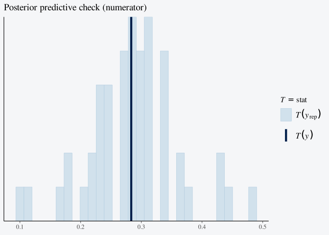
# Check distribution
pp_check(fit_zi, type = "dens_overlay")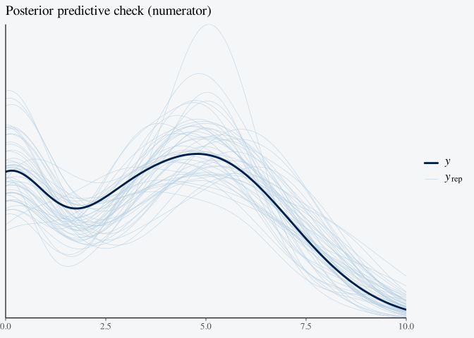
See Also
-
vignette("getting-started")- Basic usage -
vignette("spatial-temporal")- Spatial and temporal models -
?ratiod_zibinomial,?ratiod_zoibinomial- Function documentation