Mathematical Foundations

Overview

hexify implements the ISEA (Icosahedral Snyder Equal Area) discrete global grid system. This vignette explains the mathematical foundations: the projection geometry, coordinate systems, aperture subdivision, and cell indexing.

The Problem: Equal-Area Grids on a Sphere

Any projection from a sphere to a plane must distort something. For spatial statistics, we need cells of equal area regardless of location. Standard latitude-longitude grids fail badly: a 1° cell at the equator covers ~12,300 km², while the same cell near the poles covers a tiny fraction of that.

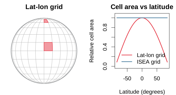
The ISEA projection solves this by:

1. Choosing a regular icosahedron with the same surface area as the sphere

2. Projecting each spherical “cap” onto its corresponding flat triangular face using a modified Lambert equal-area projection

3. Overlaying a hexagonal grid on the resulting planar triangles

The Lambert Azimuthal Equal-Area Projection

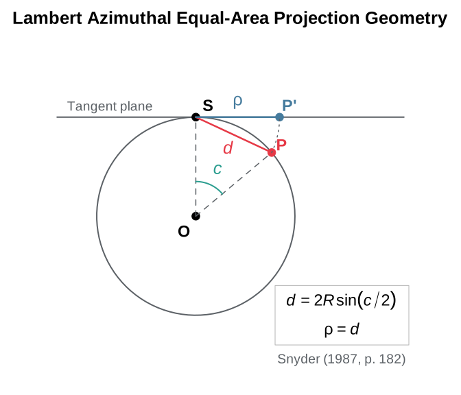
The foundation of Snyder’s projection is Lambert’s azimuthal equal-area projection, developed by Johann Heinrich Lambert in 1772. The projection maps a sphere of radius $R$ to a tangent plane while preserving area exactly (Snyder, 1987, p. 182).

Definition

The Lambert azimuthal equal-area projection is defined by a mathematical constraint, not a geometric construction. For a projection centered at point $S$:

• Azimuthal property: The direction (azimuth) from $S$ to any point $P$ on the sphere equals the direction from the origin to $P'$ on the plane

• Equal-area property: Any region on the sphere maps to a region of identical area on the plane

These two constraints uniquely determine the radial distance formula. For a point $P$ at angular distance $c$ from the center (measured along the sphere surface), the projected distance from the origin is:

$$\rho = 2R \sin\left(\frac{c}{2}\right)$$

This is not a perspective projection and has no simple geometric interpretation like “chord distance” or “ray intersection.” The formula is derived analytically from the equal-area constraint (Snyder, 1987, p. 182-185).

Forward Formulas

For the oblique aspect centered at $(\lambda_0, \phi_1)$, the full formulas are (Snyder, 1987, eq. 24-2 to 24-4, p. 185):

$$k' = \sqrt{\frac{2}{1 + \sin\phi_1\sin\phi + \cos\phi_1\cos\phi\cos(\lambda - \lambda_0)}}$$

$$x = R \cdot k' \cdot \cos\phi \cdot \sin(\lambda - \lambda_0)$$

$$y = R \cdot k' \cdot [\cos\phi_1\sin\phi - \sin\phi_1\cos\phi\cos(\lambda - \lambda_0)]$$

Equal-Area Proof

The projection preserves area because the radial and tangential scale factors satisfy $h' \cdot k' = 1$ at every point. At angular distance $c$ from center (Snyder, 1987, eq. 24-22, 24-23, p. 188):

$$h' = \cos\left(\frac{c}{2}\right), \quad k' = \sec\left(\frac{c}{2}\right)$$

Therefore $h' \cdot k' = \cos(c/2) \cdot \sec(c/2) = 1$, confirming the equal-area property.

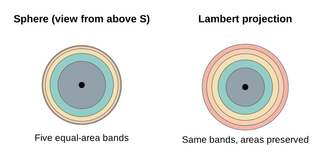
Each colored band has equal area on the sphere (the band boundaries are at $\cos\phi_i = 1 - i/5$). After Lambert projection the outer bands stretch radially and compress tangentially, and every annulus still has the same area: $\rho_i^2 = 2R^2(1 - \cos\phi_i)$ grows linearly with $i$.

Inverse Formulas

The inverse mapping $(x, y) \to (\lambda, \phi)$ recovers geographic coordinates from planar coordinates (Snyder, 1987, eq. 24-14 to 24-16, p. 187):

$$\rho = \sqrt{x^2 + y^2}$$

$$c = 2\arcsin\left(\frac{\rho}{2R}\right)$$

where $c$ is the angular distance from the projection center. Then:

$$\phi = \arcsin\left[\cos c \cdot \sin\phi_1 + \frac{y \cdot \sin c \cdot \cos\phi_1}{\rho}\right]$$

$$\lambda = \lambda_0 + \arctan\left[\frac{x \cdot \sin c}{\rho\cos\phi_1\cos c - y\sin\phi_1\sin c}\right]$$

If $\rho = 0$, the point is at the projection center: $\phi = \phi_1$, $\lambda = \lambda_0$.

Limitations

Antipode singularity: The point diametrically opposite the projection center (angular distance 180°) maps to infinity and must be excluded from the domain.

Shape distortion: While area is preserved exactly, shapes distort increasingly with distance from center. The maximum angular distortion $\omega$ at distance $c$ is (Snyder, 1987, eq. 24-24, p. 188):

$$\sin\left(\frac{\omega}{2}\right) = \frac{k'^2 - 1}{k'^2 + 1}$$

At $c = 90°$, distortion reaches $\omega \approx 70.5°$. ISEA grids limit this by using icosahedral faces subtending only ~72° from face center.

No conformality: No projection can be both equal-area and conformal (angle-preserving)—a fundamental constraint from differential geometry (Snyder, 1987, p. 16-18).

The Icosahedron

Lambert’s projection works for a single tangent plane covering at most a hemisphere. To cover the entire globe with minimal distortion, Snyder used 20 planar faces—one for each face of a regular icosahedron with the same surface area as the sphere (Snyder, 1992, p. 10).

Geometry

A regular icosahedron has:

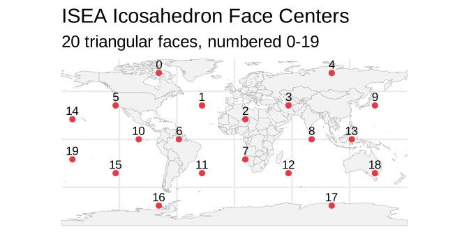
• 20 equilateral triangular faces (each covering ~1/20 of Earth’s surface)

• 12 vertices (where 5 faces meet—these become pentagon cells)

• 30 edges

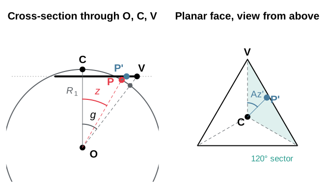
Left: the icosahedron has the same surface area as the sphere, so its face plane lies at the inradius $R_1 = 0.9104R$ from the centre O, inside the sphere, and the vertex V of the planar face lies on the ray through the sphere point at angular distance $g = 37.38°$ from the face centre C. In this cross-section the face extends from V on one side to the midpoint of the opposite edge on the other. A point P at angular distance $z$ from C maps to P’ on the face plane at radial distance $\rho$ from C. Right: on the planar face the azimuth Az’ is measured from the centre-to-vertex ray, and the three-fold symmetry of the face reduces every azimuth to one 120° sector.

Vertex Latitude Derivation

The 12 vertices are located at (Coxeter, 1973, p. 52-53):

Location	Latitude	Longitudes
North pole	+90°	0°
Upper ring	$+\arctan(1/2) \approx +26.565°$	0°, 72°, 144°, 216°, 288°
Lower ring	$-\arctan(1/2) \approx -26.565°$	36°, 108°, 180°, 252°, 324°
South pole	−90°	0°

The latitude $\arctan(1/2)$ arises from the golden ratio geometry. An icosahedron can be constructed from three mutually perpendicular golden rectangles ($1 \times \varphi$, where $\varphi = (1+\sqrt{5})/2$). The non-polar vertices have $z$-coordinate $1/s$ where $s = \sqrt{1 + \varphi^2}$, yielding $\tan\phi = 1/2$.

Standard ISEA Orientation

The default orientation places vertex 0 at longitude 11.25°, latitude $\arctan(\varphi) \approx 58.2825°$, with azimuth 0°. This places icosahedron vertices (pentagon cells) predominantly over oceans (Sahr et al., 2003, p. 123).

Snyder’s ISEA Projection

Snyder extended the Lambert projection to the icosahedron by introducing an azimuth-adjustment transformation that ensures seamless transitions between adjacent faces while maintaining the equal-area property (Snyder, 1992, p. 12).

Bradley (1946) published an approximate equal-area graticule for the icosahedron, and an editorial footnote to that paper described an exact construction by Irving Fisher. Snyder rederived Fisher’s approach and generalized it to the five Platonic solids after White, Kimerling, and Overton (1992) chose a truncated-icosahedron grid for the U.S. EPA’s EMAP global sampling design (Snyder, 1992, p. 10). ISEA is the icosahedral member of this family.

Key Constants

Constant	Symbol	Value	Source
Face center to vertex angle	$E_l$	37.37736814°	Snyder (1992, Table 1, p. 12)
Geometric angle	$G$	36°	Snyder (1992, Table 1, p. 12)
Scale factor	$R_1$	0.9103832815	Snyder (1992, eq. 5, p. 11)

The vertex angle has the closed form $\tan E_l = \sqrt{14 - 6\sqrt{5}}$ (Snyder, 1992, p. 17). $R_1$ is the radius of the icosahedron whose surface area equals that of the unit sphere: equating $20 \cdot \frac{3\sqrt{3}}{4} R_1^2 \tan^2 E_l = 4\pi$ gives $R_1 = \frac{2}{\tan E_l}\sqrt{\frac{\pi}{15\sqrt{3}}}$.

Forward Projection Steps

The complete algorithm comprises seven steps (Snyder, 1992, p. 12-13):

Step 1: Compute angular distance and azimuth from face center $(\lambda_0, \phi_0)$ to point $(\lambda, \phi)$:

$$z = \arccos(\sin\phi_0 \sin\phi + \cos\phi_0 \cos\phi \cos(\lambda - \lambda_0))$$$$\text{Az} = \arctan2(\cos\phi \sin(\lambda - \lambda_0), \cos\phi_0 \sin\phi - \sin\phi_0 \cos\phi \cos(\lambda - \lambda_0))$$

Step 2: Reduce azimuth to [0°, 120°) by exploiting 3-fold symmetry.

Step 3: Compute auxiliary angle $\delta_z$ (Snyder, 1992, eq. 9, p. 13): $$\delta_z = \arctan\left(\frac{\tan E_l}{\cos \text{Az} + \cot 30° \cdot \sin \text{Az}}\right)$$

Step 4: Compute auxiliary angle $h$ (Snyder, 1992, eq. 6, p. 12): $$h = \arccos(\sin \text{Az} \sin G \cos E_l - \cos \text{Az} \cos G)$$

Step 5: Compute adjusted azimuth $\text{Az}'$ (Snyder, 1992, eq. 7-8, p. 12): $$A_G = \text{Az} + G + h - \pi$$$$\text{Az}' = \arctan\left(\frac{2 A_G}{R_1^2 \tan^2 E_l - 2 A_G \cot 30°}\right)$$

Step 6: Compute radial distance (Snyder, 1992, eq. 10-12, p. 13): $$f = \frac{\tan E_l}{2(\cos \text{Az}' + \cot 30° \cdot \sin \text{Az}') \sin(\delta_z / 2)}$$$$\rho = 2 R_1 f \sin(z / 2)$$

Step 7: Convert to Cartesian with sector offset restored.

The Inverse Projection

The inverse projection cannot be solved analytically because the azimuth adjustment contains transcendental functions. A Newton-Raphson iteration finds the spherical azimuth Az from the planar azimuth Az’ (Snyder, 1992, eq. 20-22, p. 13):

$$f(\text{Az}) = \text{agh} - \text{Az} - G + (\pi - h) = 0$$

where $h = \arccos(\sin \text{Az} \sin G \cos E_l - \cos \text{Az} \cos G)$.

The iteration exhibits quadratic convergence, typically reaching machine precision in 3-5 iterations. hexify provides four precision modes:

Mode	Tolerance	Typical Iterations	Use Case
fast	$10^{-10}$	3-4	Interactive visualization
default	$10^{-12}$	4-5	General applications (~1 m accuracy)
high	$10^{-14}$	5-6	High-precision geodesy
ultra	$10^{-15}$	6-7	Research

Distortion

The projection is exactly equal-area, so its distortion falls on angles and local scale. On an icosahedron face the maximum angular deformation is $\omega = 17.27°$, with linear scale factors between 0.860 and 1.163 (Snyder, 1992, Table 1, p. 12). The azimuth adjustment concentrates this deformation along the three radii from the face center to its vertices, where the graticule shows visible cusps (Snyder, 1992, p. 11).

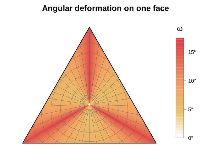
Deformation is smallest, about 5°, in the ring around the face center toward the edge midpoints, and largest along the three vertex radii, where the parallels kink as they cross. The 17.27° maximum is reached at the face center approached along a vertex radius. The Jacobian determinant of the projection equals 1 everywhere on the face, which is the equal-area property in differential form.

The Unfolded Projection

Applying the per-face projection to all 20 faces and unfolding them into a plane maps the whole sphere onto a strip of triangles (compare Snyder, 1992, Figure 12, p. 18). hexify_lonlat_to_plane() performs the composite transformation, in the same PLANE layout as dggridR’s dgGEO_to_PLANE(). Coastlines and graticule continue across every shared edge and are interrupted elsewhere:

draw_path <- function(lon, lat, col, lwd) {
  p <- hexify_lonlat_to_plane(lon, lat)
  jump <- c(FALSE, sqrt(diff(p$plane_x)^2 + diff(p$plane_y)^2) > 0.2)
  p$plane_x[jump] <- NA
  lines(p$plane_x, p$plane_y, col = col, lwd = lwd)
}

oldpar <- par(mar = c(0.5, 0.5, 2, 0.5), bg = "white")
plot(NULL, xlim = c(-0.1, 5.6), ylim = c(-0.05, 2.65), asp = 1,
     axes = FALSE, xlab = "", ylab = "", main = "Unfolded ISEA Projection")

# face outlines: side-1 triangles around each projected face centroid
centers <- hexify_face_centers()
pc <- hexify_lonlat_to_plane(centers$lon * 180/pi, centers$lat * 180/pi)
s3 <- sqrt(3)
for (f in 1:20) {
  base <- floor(pc$plane_y[f] / (s3/2)) * s3/2
  up <- (pc$plane_y[f] - base) < s3/4
  yy <- if (up) base + c(0, 0, s3/2) else base + c(s3/2, s3/2, 0)
  polygon(pc$plane_x[f] + c(-0.5, 0.5, 0), yy, border = "gray60", lwd = 0.8)
}

# 15-degree graticule
for (lon in seq(-180, 165, by = 15))
  draw_path(rep(lon, 181), seq(-90, 90, by = 1), "gray75", 0.6)
for (lat in seq(-75, 75, by = 15))
  draw_path(seq(-180, 180, by = 0.5), rep(lat, 721), "gray75", 0.6)

# coastlines
xy <- st_coordinates(st_cast(st_geometry(hexify_world), "MULTIPOLYGON"))
for (ring in split(seq_len(nrow(xy)),
                   interaction(xy[, "L1"], xy[, "L2"], xy[, "L3"], drop = TRUE)))
  draw_path(xy[ring, 1], xy[ring, 2], GREY, 0.8)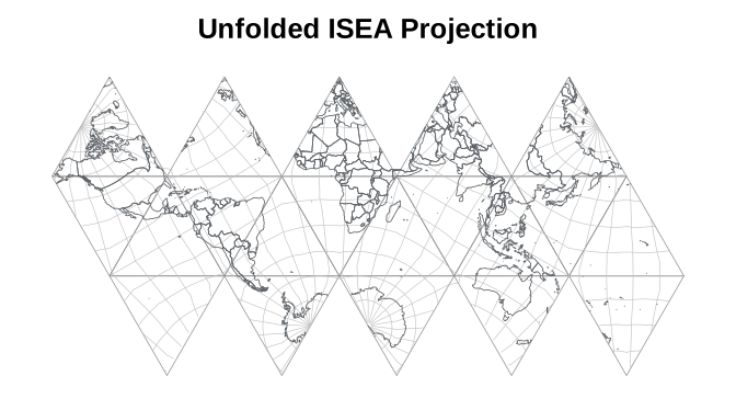

par(oldpar)

Aperture and Resolution

Aperture defines how cells subdivide at each resolution level—it’s the ratio of parent cell area to child cell area (Sahr et al., 2003, p. 124).

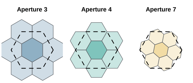
The dashed outline is the parent cell; the darker child shares its centre. For apertures 3 and 4 the parent boundary cuts through the ring children: each of the six vertex children of aperture 3 lies one third inside the parent, and each of the six edge children of aperture 4 lies half inside it, so the parent area equals $1 + 6/3 = 3$ or $1 + 6/2 = 4$ child areas. The seven aperture-7 children form a rosette with exactly the parent’s area, and its ragged boundary does not follow the parent’s edges.

Aperture Properties

Aperture	Area Ratio	Linear Scale	Rotation per Level	Orientation
3	1:3	$\sqrt{3} \approx 1.73$	30°	Alternates Class I/II
4	1:4	$2.0$	0°	Always Class I
7	1:7	$\sqrt{7} \approx 2.65$	$\arctan(\sqrt{3}/5) \approx 19.1°$	Class III

The aperture 7 rotation angle follows from the child lattice: the parent’s nearest neighbour sits at two steps along one child lattice axis plus one step along the next, a vector of length $\sqrt{7}$ child spacings at angle $\arctan\!\big(\tfrac{\sqrt{3}/2}{2 + 1/2}\big) = \arctan(\sqrt{3}/5) \approx 19.107°$ to the axis (DGGRID Manual, 2023).

Cell Count Growth

cat("Resolution  Aperture 3    Aperture 4    Aperture 7\n")
#> Resolution  Aperture 3    Aperture 4    Aperture 7
cat("---------  ----------    ----------    ----------\n")
#> ---------  ----------    ----------    ----------
for (res in 0:8) {
  cells_ap3 <- 10 * 3^res + 2
  cells_ap4 <- 10 * 4^res + 2
  cells_ap7 <- 10 * 7^res + 2
  cat(sprintf("    %d      %10s    %10s    %10s\n",
              res,
              format(cells_ap3, big.mark = ","),
              format(cells_ap4, big.mark = ","),
              format(cells_ap7, big.mark = ",")))
}
#>     0              12            12            12
#>     1              32            42            72
#>     2              92           162           492
#>     3             272           642         3,432
#>     4             812         2,562        24,012
#>     5           2,432        10,242       168,072
#>     6           7,292        40,962     1,176,492
#>     7          21,872       163,842     8,235,432
#>     8          65,612       655,362    57,648,012

Orientation Classes

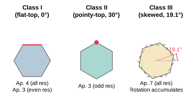
For aperture 3, orientation alternates between Class I (flat-top) and Class II (pointy-top) at each resolution. For aperture 7, each level adds a rotation of $\arctan(\sqrt{3}/5) \approx 19.1°$ (Sahr, 2008, p. 176).

Pentagon Cells

Exactly 12 cells are pentagons at every resolution. This is a topological necessity derived from Euler’s formula (Coxeter, 1973, p. 10):

$$V - E + F = 2$$

For a tiling with $h$ hexagons and $p$ pentagons on a sphere: - $V = (6h + 5p)/3$, $E = (6h + 5p)/2$, $F = h + p$

Substituting into Euler’s formula and simplifying yields $p = 12$, independent of $h$.

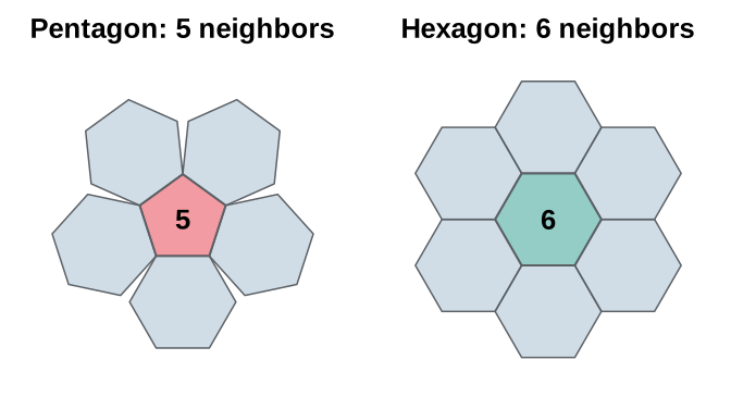
Hexagons have six neighbors; pentagons have five.

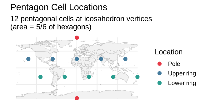
Location	Latitude	Longitudes
Poles	±90°	0°
Upper ring	$\arctan(1/2) \approx 26.57°$	0°, 72°, 144°, 216°, 288°
Lower ring	$-\arctan(1/2) \approx -26.57°$	36°, 108°, 180°, 252°, 324°

Pentagon area is exactly 5/6 of hexagonal cell area at the same resolution (Sahr et al., 2003, p. 125).

Coordinate Systems and Indexing

hexify uses a multi-stage coordinate pipeline (Sahr, 2008, p. 178):

System	Components	Description
GEO	lon, lat	WGS84 degrees
Icosa Triangle	face (0-19), tx, ty	Snyder projection output
Quad XY	quad (0-11), qx, qy	Paired-triangle coordinates
Quad IJ	quad (0-11), i, j	Quantized grid indices
Index	string	Hierarchical cell address (Z3, Z7, or Z-order)
SEQNUM	integer	Global cell ID (1-based)

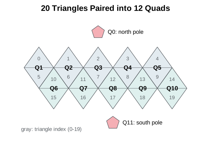
Triangle to Quad

The 20 triangular faces are paired into 12 “quads” (diamond-shaped regions). Each quad contains two adjacent triangular faces sharing an edge. This pairing transforms 20 triangles into 10 diamond-shaped quads plus 2 polar quads, simplifying grid indexing because a diamond admits a rectangular $(i, j)$ lattice (DGGRID Manual, 2023).

Quad IJ: The Integer Lattice

After Snyder projection maps a point onto a triangular face, the continuous $(x, y)$ coordinates are quantized to integer $(i, j)$ indices on the hexagonal lattice. At resolution $r$ with aperture $a$, the lattice dimension along each axis is:

$$d = \left\lfloor a^{r/2} \right\rfloor$$

The $(i, j)$ pair uniquely identifies a cell within a quad. Combined with the quad number (0–11), this gives a globally unique cell address.

Hierarchical Index Types

hexify supports three hierarchical index encodings. Each converts the $(quad, i, j)$ triple into a compact string or integer that encodes the cell’s position in the subdivision hierarchy.

Z7 Index (Aperture 7)

The Z7 index represents each cell as a hierarchical path through the aperture-7 subdivision tree (Sahr, 2025). The format is:

$$\texttt{BB}\underbrace{\texttt{D}_1\texttt{D}_2\cdots\texttt{D}_r}_{r \text{ digits}}$$

where BB is the leading field and each digit $D_k \in \{0, 1, \ldots, 6\}$ selects one of 7 children at level $k$. The digit meanings correspond to positions in the IVec3D cube coordinate system:

Digit	Direction	Meaning
0	CENTER	Center child (same position as parent)
1	K_AXES	K-axis direction
2	J_AXES	J-axis direction
3	JK_AXES	JK-axis direction
4	I_AXES	I-axis direction
5	IK_AXES	IK-axis direction
6	IJ_AXES	IJ-axis direction

The leading field is always two characters, so the resolution is nchar(index) - 2. Dropping the final digit gives the parent; appending digits 0–6 enumerates the seven positions in the next refinement level.

hexify uses a bijective Z7 variant. DGGRID’s base-cell reassignment and pentagon digit-skip rules can make its encoder non-injective near pentagons: distinct cells may receive the same string. hexify keeps the geographic quad fixed in those regions, so every cell has a distinct index and both cell -> index -> cell and index -> cell -> index round-trip.

Holding the quad fixed is what the leading field pays for. A quad is a rhombus while the aperture-7 parents are hexagons, so the quad boundary cuts through the parents of the cells along it: walking such a cell up the hierarchy arrives at one of the six neighbours of the quad’s own level-0 point rather than at the point itself. The leading field records which, as $\texttt{quad} + 12s$ with $s \in \{0, 1, \ldots, 6\}$, and a cell whose whole ancestry stays inside its quad has $s = 0$ and keeps the plain two-digit quad DGGRID writes. Recover the quad with BB %% 12, or with hexify_index_to_cell(). This matters when exchanging raw Z7 strings with DGGRID; geographic coordinates and cell geometry remain the safest interoperability layer.

# Z7 index encoding for aperture 7
g7 <- hex_grid(resolution = 4, aperture = 7)
cell <- lonlat_to_cell(16.37, 48.21, g7)
idx <- cell_to_index(cell, g7)
cat(sprintf("Cell %d -> Z7 index: %s\n", cell, idx))
#> Cell 5194 -> Z7 index: 270453
cat(sprintf("  Leading field: %s (quad %d), Digits: %s\n",
            substr(idx, 1, 2), as.integer(substr(idx, 1, 2)) %% 12L,
            substr(idx, 3, nchar(idx))))
#>   Leading field: 27 (quad 3), Digits: 0453

# Hierarchical property: parent is obtained by dropping the last digit
parent_idx <- substr(idx, 1, nchar(idx) - 1)
parent_info <- hexify_index_to_cell(parent_idx, 7, "z7")
cat(sprintf("  Parent index: %s (face %d, i=%d, j=%d)\n",
            parent_idx, parent_info$face,
            as.integer(parent_info$i), as.integer(parent_info$j)))
#>   Parent index: 27045 (face 3, i=9, j=19)

# A valid Z7 index decodes and re-encodes without changing
decoded <- hexify_index_to_cell(idx, 7, "z7")
stopifnot(identical(
  hexify_cell_to_index(decoded$face, decoded$i, decoded$j,
                       decoded$resolution, 7, "z7"),
  idx
))

Z3 Index (Aperture 3)

The Z3 index encodes the aperture-3 subdivision hierarchy using digit pairs (Sahr, 2008). Because aperture 3 alternates between Class I and Class II orientation at each level, the encoding uses two digits per resolution-level pair:

$$\texttt{BB}\underbrace{\texttt{D}_1\texttt{D}_2\texttt{D}_3\texttt{D}_4\cdots}_{2\lceil r/2 \rceil \text{ digits}}$$

Each $(i_d, j_d)$ digit pair is mapped through a lookup table to a Z3 code pair. For example, the offset $(1, 0)$ maps to digits “01”, while $(0, 1)$ maps to “22”. This mapping preserves the space-filling curve property, ensuring hierarchical locality.

# Z3 index encoding for aperture 3
g3 <- hex_grid(resolution = 8, aperture = 3)
cell <- lonlat_to_cell(16.37, 48.21, g3)
idx <- cell_to_index(cell, g3)
cat(sprintf("Cell %d -> Z3 index: %s\n", cell, idx))
#> Cell 14092 -> Z3 index: 0321202211
cat(sprintf("  Base cell: %s, Digits: %s (%d digit pairs)\n",
            substr(idx, 1, 2), substr(idx, 3, nchar(idx)),
            (nchar(idx) - 2) / 2))
#>   Base cell: 03, Digits: 21202211 (4 digit pairs)

Z-Order Index (Morton Curve)

The Z-order (Morton) index uses bit-interleaving of the $(i, j)$ coordinates, producing a Morton space-filling curve (Morton, 1966). The encoding depends on the aperture:

• Aperture 4: Binary interleaving. Each $(i, j)$ digit pair in base 2 produces one output digit: $d = 2i_b + j_b$, yielding digits in $\{0, 1, 2, 3\}$.

• Aperture 3: Base-3 interleaving. The $(i, j)$ coordinates are expressed in base 3, and digits alternate: $i_0, j_0, i_1, j_1, \ldots$

• Aperture 7: Base-7 interleaving with 2 digits per level.

# Z-order index for aperture 4
g4 <- hex_grid(resolution = 8, aperture = 4)
cell <- lonlat_to_cell(16.37, 48.21, g4)
idx <- cell_to_index(cell, g4)
cat(sprintf("Aperture 4: Cell %d -> Z-order index: %s\n", cell, idx))
#> Aperture 4: Cell 140534 -> Z-order index: 0311310300

Index Type Comparison

Property	Z7	Z3	Z-order
Apertures	7 only	3 only	3, 4, 7
Digits per level	1 (range 0–6)	2 (pairs)	1 (ap3/4) or 2 (ap7)
Encoding	Hierarchical path	Mapping table	Bit interleaving
Locality	Excellent	Excellent	Good
Parent operation	Drop last digit	Drop last pair	Drop last digit(s)
Index length (res $r$)	$2 + r$	$2 + 2\lceil r/2\rceil$	$2 + r$ or $2 + 2r$

All three hexify encodings are bijective: each valid $(quad, i, j)$ cell maps to exactly one index string, and vice versa. hexify stores indices as character strings to support arbitrary precision and avoid integer overflow at high resolutions. As noted above, hexify’s bijective Z7 strings intentionally differ from DGGRID in the pentagon regions where DGGRID’s raw Z7 encoding collides.

SEQNUM: The Flat Cell ID

The SEQNUM provides a unique integer for each cell, independent of the hierarchical index. The total cell count at resolution $r$ with aperture $a$ is:

$$N(r) = 10 \times a^r + 2$$

The “+2” accounts for the two polar pentagon cells. SEQNUMs are assigned by traversing quads in order (0–11) and cells within each quad in row-major $(i, j)$ order. This numbering maintains compatibility with dggridR.

Compact uint64 Storage

For database-friendly storage, hexify can pack any hierarchical index into a single 64-bit unsigned integer:

$$\texttt{uint64} = (\texttt{face} \ll 60) \;|\; \texttt{packed\_digits}$$

The top 4 bits encode the face (0–11), and the remaining 60 bits pack the index digits. This supports resolutions up to $\lfloor 60 / \lceil\log_2 a\rceil \rfloor$ before overflow.

H3 Comparison

hexify supports Uber’s H3 system as a first-class alternative to the ISEA backend. H3 uses a fundamentally different design with important trade-offs.

Architecture

Property	ISEA (hexify native)	H3 (Uber)
Projection	Snyder ISEA (equal-area)	Face-centered gnomonic
Polyhedron	Icosahedron (20 faces)	Icosahedron (20 faces)
Aperture	3, 4 and 7 in any sequence	7 (fixed)
Cell area	Exactly equal	Varies by location
Resolutions	0–30	0–15
Cell IDs	Integer SEQNUM	64-bit hex string
Pentagon handling	12 per resolution	12 per resolution

Both systems tile the sphere with hexagons on an icosahedral framework, but the projection and subdivision choices lead to different properties.

The Area Variation Trade-Off

The most significant difference is area uniformity. ISEA uses the Snyder equal-area projection, guaranteeing that all hexagonal cells at a given resolution have identical area (pentagons are 5/6 of hex area). H3 uses a gnomonic (central) projection per face, which is not equal-area. This causes cell areas to vary by latitude:

# Compare ISEA (constant area) vs H3 (variable area) at similar resolutions
lats <- seq(-85, 85, by = 5)
lons <- rep(10, length(lats))

# ISEA: aperture 7, resolution 6 (~130 km² cells)
g_isea <- hex_grid(resolution = 6, aperture = 7)
isea_cells <- lonlat_to_cell(lons, lats, g_isea)
isea_areas <- cell_area(isea_cells, g_isea)

# H3: resolution 4 (~1,770 km² cells — different scale, but shows the pattern)
g_h3 <- hex_grid(resolution = 4, type = "h3")
#> H3 cells are not exactly equal-area; hexagon area varies ~2x within a resolution.
#> This message is displayed once per session.
h3_cells <- lonlat_to_cell(lons, lats, g_h3)
h3_areas <- cell_area(h3_cells, g_h3)

# Normalize to show relative variation
isea_rel <- isea_areas / mean(isea_areas)
h3_rel <- h3_areas / mean(h3_areas)

oldpar <- par(mar = c(4, 4, 2, 1), bg = "white")
plot(lats, h3_rel, type = "l", col = "#E63946", lwd = 2.5,
     xlab = "Latitude (degrees)", ylab = "Relative cell area",
     main = "Cell Area Variation by Latitude",
     ylim = range(c(isea_rel, h3_rel)))
lines(lats, isea_rel, col = "#457B9D", lwd = 2.5)
abline(h = 1, lty = 2, col = GREY)
legend("bottomleft", legend = c("H3 (gnomonic)", "ISEA (equal-area)"),
       col = c("#E63946", "#457B9D"), lwd = 2.5, bty = "n")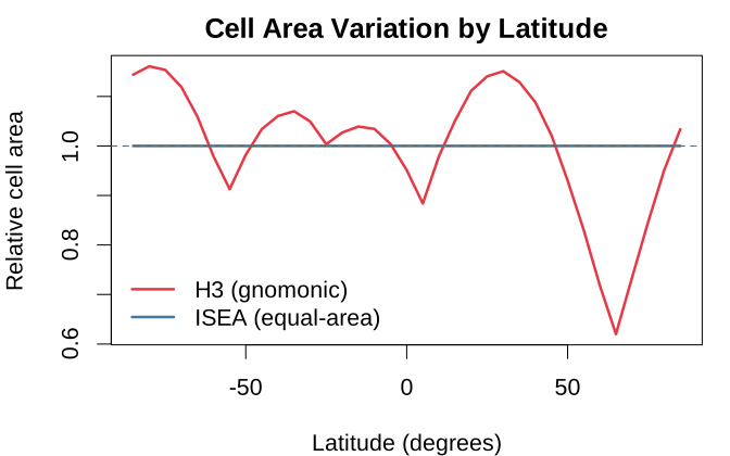

par(oldpar)

For ecological and statistical applications where equal-area cells are important (species density estimation, spatial sampling), ISEA is the correct choice. For applications where hierarchical indexing speed matters more than area equality (ride-sharing, logistics), H3 may be preferable.

Resolution Mapping

Because ISEA supports multiple apertures, there is no one-to-one resolution mapping to H3. The h3_crosswalk() function finds the closest H3 resolution for a given ISEA grid:

# H3 resolution table: compare H3 and ISEA aperture-7 cell areas
cat("H3 Res  Avg Area (km²)  ISEA Ap7 Equivalent\n")
#> H3 Res  Avg Area (km²)  ISEA Ap7 Equivalent
cat("------  --------------  -------------------\n")
#> ------  --------------  -------------------
for (h3_res in 0:8) {
  g_h3 <- hex_grid(resolution = h3_res, type = "h3")
  h3_area <- g_h3@area_km2

  # Find closest ISEA ap7 resolution by brute force
  best_res <- 0
  best_diff <- Inf
  for (r in 0:15) {
    g_test <- hex_grid(resolution = r, aperture = 7)
    d <- abs(log(g_test@area_km2) - log(h3_area))
    if (d < best_diff) { best_diff <- d; best_res <- r }
  }
  g_isea <- hex_grid(resolution = best_res, aperture = 7)
  cat(sprintf("   %2d   %14.1f  res %d (%.1f km²)\n",
              h3_res, h3_area, best_res, g_isea@area_km2))
}
#>     0        4357449.4  res 1 (7084244.7 km²)
#>     1         609788.4  res 2 (1036718.7 km²)
#>     2          86801.8  res 3 (148620.5 km²)
#>     3          12393.4  res 4 (21242.1 km²)
#>     4           1770.3  res 5 (3034.8 km²)
#>     5            252.9  res 6 (433.5 km²)
#>     6             36.1  res 7 (61.9 km²)
#>     7              5.2  res 8 (8.8 km²)
#>     8              0.7  res 9 (1.3 km²)

When to Use Which

Use case	Recommended	Reason
Species distribution modeling	ISEA	Equal area eliminates sampling bias
Spatial statistics (Moran’s I, variograms)	ISEA	Equal area ensures unbiased estimates
Ride-sharing / logistics	H3	Fast hierarchical lookups
Visualization only	Either	Area variation invisible at map scale
Cross-system interoperability	Both via h3_crosswalk()	Bidirectional mapping

Round-Trip Accuracy

original_lon <- 16.37
original_lat <- 48.21

cat(sprintf("Original: (%.4f, %.4f)\n\n", original_lon, original_lat))
#> Original: (16.3700, 48.2100)

for (ap in c(3, 4, 7)) {
  res <- if (ap == 7) 6 else 10
  grid <- hex_grid(resolution = res, aperture = ap)
  cell_id <- lonlat_to_cell(original_lon, original_lat, grid)
  recovered <- cell_to_lonlat(cell_id, grid)
  error_km <- sqrt((recovered$lon - original_lon)^2 +
                   (recovered$lat - original_lat)^2) * 111
  cat(sprintf("Aperture %d (res %2d): cell %d -> (%.4f, %.4f), ~%.1f km from center\n",
              ap, res, cell_id,
              recovered$lon, recovered$lat, error_km))
}
#> Aperture 3 (res 10): cell 126594 -> (16.4204, 48.2877), ~10.3 km from center
#> Aperture 4 (res 10): cell 2245587 -> (16.4177, 48.2119), ~5.3 km from center
#> Aperture 7 (res  6): cell 252091 -> (16.3388, 48.2019), ~3.6 km from center

Summary of ISEA Properties

Property	Description
Equal area	All hexagonal cells identical; pentagons = 5/6 hex area
Bounded distortion	Max angular distortion ~17.3° at face edges
Uniform topology	Hexagons have 6 neighbors; pentagons have 5
12 pentagons	Topological necessity from Euler’s formula

References

• Brodsky, I. (2018). H3: Uber’s Hexagonal Hierarchical Spatial Index. Uber Engineering Blog.

• H3 documentation (2024). H3: A Hexagonal Hierarchical Geospatial Indexing System. https://h3geo.org/

• Bradley, A.D. (1946). Equal-area projection on the icosahedron. Geographical Review, 36(1), 101-104.

• Coxeter, H.S.M. (1973). Regular Polytopes (3rd ed.). Dover Publications.

• DGGRID Manual (2023). DGGRID Version 7.8 Documentation. https://github.com/sahrk/DGGRID

• Morton, G.M. (1966). A Computer Oriented Geodetic Data Base and a New Technique in File Sequencing. IBM Technical Report.

• Sahr, K. (2008). Location coding on icosahedral aperture 3 hexagon discrete global grids. Computers, Environment and Urban Systems, 32(3), 174-187.

• Sahr, K. (2025). IGEO7: An equal-area hierarchical hexagonal discrete global grid system with Z7 indexing. Cartography and Geographic Information Science.

• Sahr, K., White, D., & Kimerling, A.J. (2003). Geodesic Discrete Global Grid Systems. Cartography and Geographic Information Science, 30(2), 121-134.

• Snyder, J.P. (1987). Map Projections: A Working Manual. U.S. Geological Survey Professional Paper 1395.

• Snyder, J.P. (1992). An equal-area map projection for polyhedral globes. Cartographica, 29(1), 10-21.

• White, D., Kimerling, A.J., & Overton, W.S. (1992). Cartographic and geometric components of a global sampling design for environmental monitoring. Cartography and Geographic Information Systems, 19(1), 5-22.