Lambert's Construction of Snyder's Projection

Gilles Colling

2026-10-10

Snyder’s projection (Snyder 1992) maps each face of the icosahedron, as a spherical triangle, onto a plane triangle of the same area. Snyder built it from Lambert’s azimuthal equal-area projection centred on the face, and changed the azimuths and radii of that projection so that the face fills the triangle exactly. Lambert’s projection has a construction with compass and ruler. In this article I follow the points of one face through that construction and through Snyder’s change of it, step by step, with three functions:

• projection_stages() returns each point’s place at every step;
• projection_distortion(stage = ) returns Tissot’s indicatrix at every step;
• hex_globe(lambert = ) draws the steps on a globe, with a slider.

The sphere has radius 1 throughout. For a face, T is its centre on the sphere, S a point of the face, z the arc from T to S, and Az the azimuth of S seen from T, measured from the face’s first vertex.

Installation

# Install from CRAN
install.packages("hexify")

# Or install development version from GitHub
# install.packages("pak")
pak::pak("gcol33/hexify")

One point

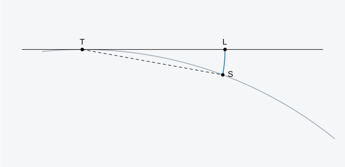
Lambert’s projection is built on the plane that touches the sphere at T. The point S lies on a circle with centre T and radius |TS|, in the plane that holds S and the normal of the sphere at T. S swings along that circle down onto the touching plane, and lands at the Lambert point L, so that

$$|TL| = |TS| = 2 \sin(z / 2).$$

L keeps the azimuth of S. projection_stages() returns the point’s plane coordinates u and v at each step, along the x and y axes of the face’s triangle, from the face centre:

s <- projection_stages(grid, lon = 20, lat = 40)
s[, c("face", "arc", "az", "lambert_u", "lambert_v")]
#>   face      arc      az lambert_u lambert_v
#> 1    2 20.50369 19.4326 0.1184239 0.3356732
c(TL = sqrt(s$lambert_u^2 + s$lambert_v^2), chord = 2 * sin(s$arc * pi / 360))
#>        TL     chord 
#> 0.3559504 0.3559504

The figure shows the construction in the plane of S, T and the sphere’s centre: the sphere’s circle, the touching plane at T (the horizontal line at height 1), and the circle about T that S swings along.

One face

Every point of the face swings down the same way. The face lands on the touching plane as a triangle whose edges are curved: its corners lie at distance 0.6409 from T, and the middle of each edge farther out than the straight line between two corners. Lambert’s projection is equal-area, so this curved triangle has the face’s area, 4 * pi / 20 = 0.6283, and every cell keeps its area.

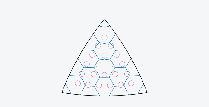
The ellipses are Tissot’s indicatrices: the images of small circles of equal size on the sphere. On Lambert’s projection, at arc z from the centre, a circle is stretched by $1 / \cos(z / 2)$ across the radius and shrunk by $\cos(z / 2)$ along it, so its area does not change:

corner <- projection_stages(grid, lon = 11.25, lat = 58.282525588538995, face = 0L)
d <- projection_distortion(grid, c(20, 11.25), c(40, 58.282525588538995), stage = "lambert")
d[, c("a", "b", "areal", "angular")]
#>          a         b areal  angular
#> 1 1.016224 0.9840350     1 1.844139
#> 2 1.055661 0.9472736     1 6.204086

The second row is a corner of the face (a vertex of the icosahedron, z = 37.38 degrees), where Lambert’s projection deforms angles most on the face, by 6.2 degrees.

Cells that lie wholly on the face keep their area on the curved triangle. For this grid’s hexagons on the face, their areas there over their areas on Snyder’s plane triangle, which are their areas on the sphere:

paths <- hexify:::grid_surface_paths(grid, NULL, 0.002)
rows <- split(seq_len(nrow(paths)), paths[, "cell"])
inside <- vapply(rows, function(i) all(paths[i, "face"] == 0), logical(1))
inside <- inside & !is_pentagon(as.numeric(names(rows)), grid)
sum(inside)
#> [1] 5
cell_area <- function(i, stage) {
  ll <- hexify:::vec_lonlat(paths[i, c("sphere_x", "sphere_y", "sphere_z")])
  st <- projection_stages(grid, ll[, 1], ll[, 2], face = 0L)
  u <- st[[paste0(stage, "_u")]]
  v <- st[[paste0(stage, "_v")]]
  abs(sum(u * c(v[-1], v[1]) - c(u[-1], u[1]) * v)) / 2
}
range(vapply(rows[inside], cell_area, numeric(1), stage = "lambert") /
        vapply(rows[inside], cell_area, numeric(1), stage = "snyder"))
#> [1] 0.9999848 1.0000005

The walls are drawn through points 0.002 radians apart on the sphere, and the ratios differ from 1 by that sampling only.

The edges of the curved triangle are not those of a plane triangle, so the faces of the icosahedron do not fit together on Lambert’s projection, and cells there that cross a face edge do not close up.

The nudge

Snyder changes Lambert’s projection within the touching plane. He moves the point from the azimuth Az to an azimuth Az’ and multiplies its radius by a factor f, which depends on the azimuth only:

$$\rho = 2 f \sin(z / 2).$$

He chooses Az’ so that the ray from the centre at Az’ cuts off as much area of the plane triangle as the ray at Az cuts off of the face, in each of the six right triangles between the centre, a corner and the middle of an edge (Snyder 1992, eqs. 6 to 11), and f so that the face edge lands on the triangle’s edge. I call the new point N, the nudged point. The figure shows the curved triangle in grey and the straight one the nudge makes of it, with an arrow from L to N at points of the face.

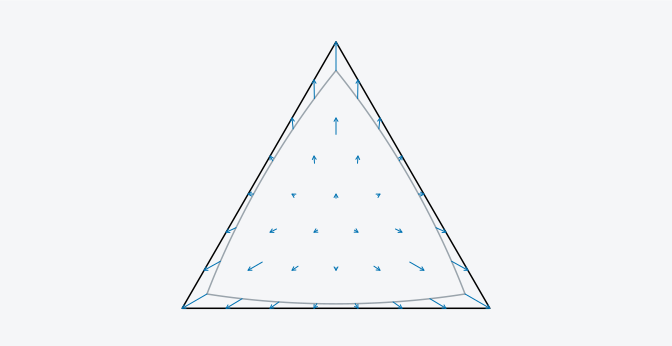
How far the nudge moves the points, over a lattice of points 60 steps to a face edge. Snyder’s projection is equal-area, so a lattice on the plane triangle spreads the points evenly over the face’s area:

ll <- face_lattice(grid, 60)
dense <- projection_stages(grid, ll[, 1], ll[, 2], face = 0L)
r1 <- attr(dense, "r1")
edge <- sqrt(16 * pi / (sqrt(3) * 20)) / r1
moved <- sqrt((dense$nudge_u - dense$lambert_u)^2 +
              (dense$nudge_v - dense$lambert_v)^2) / edge
turn <- abs((dense$az_prime - dense$az + 180) %% 360 - 180)
c(largest = max(moved), mean = mean(moved), largest_turn_deg = max(turn))
#>          largest             mean largest_turn_deg 
#>       0.09301926       0.03064207       1.90403522

moved is |LN| over the edge of the nudged triangle. The largest is at the corners. paper/bench/bench_lambert_nudge.R measures the same over 20,301 points and on the octahedron. The nudge moves the corners by about a tenth of an edge, which shows on a globe without magnification, and the points near the centre by much less.

The nudge keeps areas in proportion: the nudged triangle has $1 / R'^2$ = 1.2066 times the face’s area, everywhere on it. It does not keep the shape of Tissot’s ellipses. Snyder’s projection bends along the three lines from the centre to the corners (Snyder 1992, p. 11): the ellipses on the two sides of such a line differ, and a line on the sphere that crosses it gets a kink there.

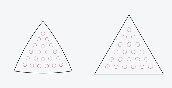
On the left Lambert’s ellipses, on the right those after the nudge, at the same points. The largest angular deformation after the nudge is at the centre, approached along the lines to the corners, 17.27 degrees (Snyder 1992, Table 1):

centre <- hexify:::cpp_face_xy_to_ll(hexify:::icosa_arg(grid), 0.5,
                                     1 / (2 * sqrt(3)) + 1e-7, 0L)
projection_distortion(grid, centre[1], centre[2], stage = "nudge")[, c("a", "b", "angular")]
#>          a         b  angular
#> 1 1.277792 0.9442593 17.26559

The scaling

The last step scales the touching plane about the sphere’s centre by $R'$ = 0.9104. This takes the plane at distance 1 from the centre onto the face plane, at distance $R'$, and the nudged triangle onto the plane triangle with the face’s area. It is Snyder’s projection: $\rho = 2 R' f \sin(z / 2)$. The scaling multiplies every length by $R'$, so Tissot’s ellipses keep their shape and the areal scale becomes 1.

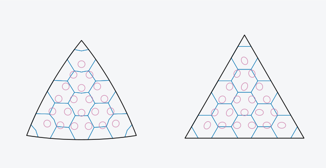
The last step is the forward projection itself: tx and ty of projection_stages() are the triangle coordinates hexify_forward() gives.

p <- hexify_forward(20, 40)
c(p[["icosa_triangle_x"]] - s$tx, p[["icosa_triangle_y"]] - s$ty)
#> [1] 0 0

Fuller’s projection beside it

Fuller’s projection (projection = "fuller") maps the same face onto the same triangle without Lambert’s projection behind it, and is not equal-area. The figure shows the face under Snyder’s projection (left) and Fuller’s (right), with Tissot’s ellipses of each at the same points.

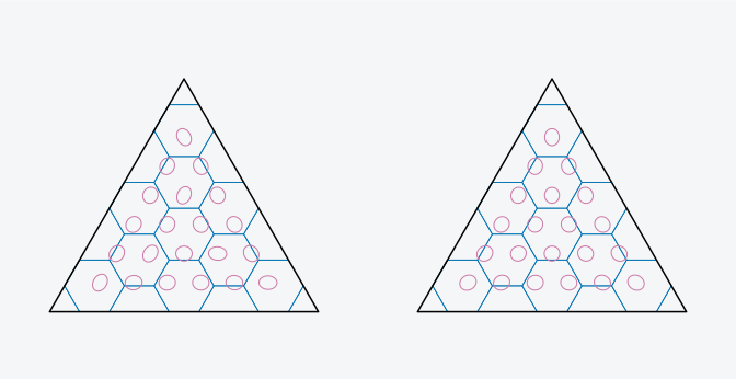
Over 5,000 random points of the sphere, the range of the areal scale and the largest angular deformation of each:

set.seed(1)
lon <- runif(5000, -180, 180)
lat <- asin(runif(5000, -1, 1)) * 180 / pi
df <- projection_distortion(fuller, lon, lat)
ds <- projection_distortion(grid, lon, lat)
rbind(snyder = c(range(ds$areal), max_angular = max(ds$angular)),
      fuller = c(range(df$areal), max_angular = max(df$angular)))
#>                           max_angular
#> snyder 1.0000000 1.000000    17.14866
#> fuller 0.9506552 1.076505    13.06439

All faces

On the globe every face swings down onto its own touching plane, so the faces come apart along their edges, and the gaps close again only on the solid. hex_globe(lambert = ) opens the globe at a step of the construction, from 0 (the sphere) through 1 (the Lambert points) and 2 (the nudged points) to 3 (the faces); the slider moves along it. The globes need a browser with WebGPU (see the Interactive Globe article).

hex_globe(grid, lambert = 1, center = c(lon = 20, lat = 40),
          width = "100%", height = 560)

At step 1 the curved triangles of the faces leave gaps between them, and coastlines and cell walls stop at the face edges. Moving the slider to 2 straightens the edges; at 3 the faces close into the icosahedron whose faces have the area of theirs on the sphere, whose corners lie 1.1456 radii from the centre, outside the sphere.

One path

The menu beside the slider switches from the three steps to one path per point: the angle below the touching plane, the azimuth, the radius and the height of the plane change together, so that the point leaves S along the compass circle and lands on Snyder’s point.

hex_globe(grid, lambert = 0, lambert_path = "single", land = TRUE,
          width = "100%", height = 560)

Earlier pictures of the construction

Wikipedia’s article on Lambert’s projection describes the construction with the circle centred at the point of tangency and draws it in a cross-section figure; it also has an animation in which the sphere opens at a pole into a disc while every cell of a grid keeps its area (https://en.wikipedia.org/wiki/Lambert_azimuthal_equal-area_projection, read 2026-10-10). Snyder (1992) describes his projection as Lambert’s azimuthal equal-area projection with the azimuths and the radial distances adjusted. In web searches on 2026-10-10 I did not find an animation that carries out Lambert’s construction face by face on a polyhedron or shows Snyder’s adjustment as a step of its own.

Reference

Snyder, J. P. (1992). An equal-area map projection for polyhedral globes. Cartographica 29(1), 10-21. https://doi.org/10.3138/27H7-8K88-4882-1752