ggguides

Simple, Intuitive Legend Control for ggplot2

The ggguides package provides one-liner functions for common legend operations in ggplot2. Instead of memorizing theme() arguments and guide specifications, use readable functions like legend_left(), legend_style(), and legend_inside() to position, style, and customize legends with minimal code.

Quick Start

library(ggplot2)
library(ggguides)

p <- ggplot(mtcars, aes(mpg, wt, color = factor(cyl))) +
  geom_point(size = 3)

# Position legends
p + legend_left()
p + legend_inside("topright")

# Style legends
p + legend_style(size = 14, title_face = "bold")

# Combine freely
p + legend_bottom() + legend_style(background = "grey95")

Example

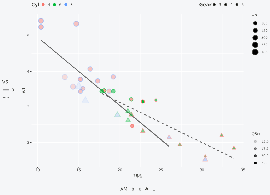
Six legends on four sides, each one positioned and styled independently. ggplot2 lets several legends share a side; ggguides lets you pick which legend goes where, slide it along the rail, and style it without touching the others.

p6 +
  # Side placement. Two legends share the top rail, two share the right.
  legend_top(by = "colour")    + legend_top(by = "fill")     +
  legend_right(by = "size")    + legend_right(by = "alpha")  +
  legend_bottom(by = "shape")  + legend_left(by = "linetype") +

  # Slide each one along its rail.
  legend_style(by = "colour",   justification = "left")   +
  legend_style(by = "fill",     justification = "right")  +
  legend_style(by = "size",     justification = "top")    +
  legend_style(by = "alpha",    justification = "bottom") +

  # Appearance (bold titles, smaller keys, smaller text, forced direction).
  legend_style(by = "colour", title_face = "bold",
               key_width = 0.4, key_height = 0.4) +
  legend_style(by = "size",   title_size = 9, size = 8)  +
  legend_style(by = "shape",  direction = "horizontal")

legend_style(by = ...) calls are additive, so one line per parameter is the intended shape. Full walkthrough in the Multiple Legends vignette.

Statement of Need

Legend customization in ggplot2 often requires verbose theme() calls with non-obvious argument names (legend.position, legend.justification, legend.box.just), and guide specifications scattered across guides() and scale_*() functions. Common tasks like positioning a legend inside the plot, styling the legend box, or managing multiple legends require looking up documentation repeatedly.

ggguides addresses this by providing:

• Readable function names that describe what they do (legend_left(), legend_inside(), legend_reverse())
• Sensible defaults that handle related settings together (e.g., legend_left() sets position, justification, and box alignment)
• Consistent API across positioning, styling, and multi-legend operations
• Patchwork integration for multi-panel figures with shared legends

Installation

install.packages("ggguides")

Or install the development version from GitHub:

# install.packages("pak")
pak::pak("gcol33/ggguides")

Features

Position Functions

• legend_left() / legend_right(): Side positioning with proper alignment
• legend_top() / legend_bottom(): Horizontal layout with optional plot alignment
• legend_inside(): Position inside plot using coordinates or shortcuts ("topright", "bottomleft", etc.)
• legend_none(): Remove legend entirely

Style Functions

• legend_style(): Comprehensive styling (size, font, background, borders, margins)
• legend_wrap(): Wrap entries into columns or rows
• legend_reverse(): Reverse entry order
• legend_order(): Reorder legend entries
• legend_keys(): Customize key appearance
• colorbar_style(): Style continuous color legends

Multiple Legend Control

• legend_hide() / legend_select(): Show/hide specific legends by aesthetic
• legend_order_guides(): Control display order of multiple legends
• legend_merge() / legend_split(): Combine or separate legend entries
• by parameter: Apply any function to specific aesthetics only

Multi-Panel Support

• collect_legends(): Collect legends from patchwork compositions
• collect_axes(): Collect axes from patchwork compositions
• shared_legend(): Combine plots with shared legend (no patchwork required)
• get_legend(): Extract legend as standalone grob

Usage Examples

Position Helpers

library(ggplot2)
library(ggguides)

p <- ggplot(mtcars, aes(mpg, wt, color = factor(cyl))) +
  geom_point(size = 3) +
  labs(color = "Cylinders")

legend_left() / legend_right()

Position with proper alignment (sets justification and box.just together):

p + legend_left()
p + legend_right()

legend_top() / legend_bottom()

Horizontal layout with optional plot alignment:

p + legend_top()
p + legend_bottom()

# Align to full plot (useful with titles)
p + labs(title = "My Title") + legend_top(align_to = "plot")

legend_inside()

Position inside the plot using coordinates or shortcuts:

# Using shortcuts
p + legend_inside(position = "topright")
p + legend_inside(position = "bottomleft")

# Using coordinates
p + legend_inside(x = 0.95, y = 0.95, justification = c("right", "top"))

# With custom styling
p + legend_inside(position = "center", background = "grey95", border = "grey50")

legend_none()

Remove the legend entirely:

p + legend_none()

---

Style Helpers

legend_style()

Comprehensive styling in one call:

# Change font size - affects both title and labels
p + legend_style(size = 14)

# Change font family
p + legend_style(family = "serif")
p + legend_style(family = "mono")

# Combine size and family
p + legend_style(size = 14, family = "serif")

# Full styling with title emphasis
p + legend_style(
  size = 12,
  title_size = 14,
  title_face = "bold",
  key_width = 1.5,
  background = "grey95",
  background_color = "grey70",
  margin = 0.3
)

legend_wrap()

Wrap legend entries into columns or rows:

ggplot(mpg, aes(displ, hwy, color = class)) +
  geom_point() +
  legend_wrap(ncol = 2)

# Or by rows
ggplot(mpg, aes(displ, hwy, color = class)) +
  geom_point() +
  legend_wrap(nrow = 2)

legend_reverse()

Reverse legend entry order:

p + legend_reverse()

---

Multiple Legends

When a plot has multiple aesthetics, control each legend separately:

legend_hide() / legend_select()

Hide specific legends or keep only certain ones:

# Plot with multiple aesthetics
p <- ggplot(mtcars, aes(mpg, wt, color = factor(cyl), size = hp)) +
  geom_point() +
  labs(color = "Cylinders", size = "Horsepower")

# Hide the size legend
p + legend_hide(size)

# Keep only the colour legend
p + legend_select(colour)

Position legends separately

Use the by parameter to position legends independently:

# Colour legend on left, size legend at bottom
p +
  legend_left(by = "colour") +
  legend_bottom(by = "size")

Style legends separately

Apply different styles to different legends:

p +
  legend_style(title_face = "bold", by = "colour") +
  legend_style(size = 10, by = "size")

legend_order_guides()

Control the display order of multiple legends:

# Size legend first, then colour
p + legend_order_guides(size = 1, colour = 2)

---

Patchwork Integration

collect_legends()

Collect legends from patchwork compositions:

library(patchwork)

p1 <- ggplot(mtcars, aes(mpg, wt, color = factor(cyl))) +
  geom_point() + labs(title = "Plot 1")
p2 <- ggplot(mtcars, aes(mpg, hp, color = factor(cyl))) +
  geom_point() + labs(title = "Plot 2")

# Without collection (duplicate legends)
p1 | p2

# With collection
collect_legends(p1 | p2)

# Position at bottom
collect_legends(p1 | p2, position = "bottom")

Height Spanning

For stacked plots, use span = TRUE to make the legend span the full height. Using different plot heights makes the spanning behavior more visible:

library(patchwork)

p3 <- ggplot(mtcars, aes(mpg, disp, color = factor(cyl))) +
  geom_point() + labs(title = "Plot 3")

# Stack with different heights: 4, 2, 1
stacked <- (p1 / p2 / p3) + plot_layout(heights = c(4, 2, 1))

# Default: legend centered
collect_legends(stacked, position = "right")

# With spanning: legend fills full height
gt <- collect_legends(stacked, position = "right", span = TRUE)
grid::grid.draw(gt)

Row-Specific Attachment

Attach the legend to specific rows instead of spanning all:

# Attach legend to row 1 only (the tallest plot)
gt <- collect_legends(stacked, position = "right", span = 1)
grid::grid.draw(gt)

# Attach legend to rows 1 and 2
gt <- collect_legends(stacked, position = "right", span = 1:2)
grid::grid.draw(gt)

---

Combining Functions

Functions compose naturally:

ggplot(mpg, aes(displ, hwy, color = class)) +
  geom_point() +
  legend_left() +
  legend_style(size = 12, title_face = "bold", background = "grey95")

ggplot(mpg, aes(displ, hwy, color = class)) +
  geom_point() +
  legend_wrap(ncol = 2) +
  legend_bottom()

---

cowplot / Base Grid Support

ggguides also works without patchwork for cowplot users or anyone using base grid:

get_legend()

Extract a legend as a standalone grob:

p <- ggplot(mtcars, aes(mpg, wt, color = factor(cyl))) +
  geom_point() + labs(color = "Cylinders")

# Extract the legend
leg <- get_legend(p)

# Use with cowplot::plot_grid() or grid::grid.draw()
grid::grid.draw(leg)

shared_legend()

Combine plots with a shared legend (no patchwork required):

p1 <- ggplot(mtcars, aes(mpg, wt, color = factor(cyl))) +
  geom_point() + labs(title = "Plot 1", color = "Cylinders")
p2 <- ggplot(mtcars, aes(mpg, hp, color = factor(cyl))) +
  geom_point() + labs(title = "Plot 2", color = "Cylinders")
p3 <- ggplot(mtcars, aes(mpg, disp, color = factor(cyl))) +
  geom_point() + labs(title = "Plot 3", color = "Cylinders")

# Side-by-side with shared legend
gt <- shared_legend(p1, p2, ncol = 2, position = "right")
grid::grid.draw(gt)

# Stacked with legend at bottom
gt <- shared_legend(p1, p2, p3, ncol = 1, position = "bottom")
grid::grid.draw(gt)

# 2x2 grid
gt <- shared_legend(p1, p2, p3, p1, ncol = 2, nrow = 2, position = "right")
grid::grid.draw(gt)

All ggguides styling functions (legend_style(), legend_wrap(), etc.) work on individual plots regardless of layout package.

Documentation

• Getting Started
• Positioning
• Styling
• Multiple Legends
• Patchwork Integration

Support

“Software is like sex: it’s better when it’s free.” — Linus Torvalds

I’m a PhD student who builds R packages in my free time because I believe good tools should be free and open. I started these projects for my own work and figured others might find them useful too.

If this package saved you some time, buying me a coffee is a nice way to say thanks. It helps with my coffee addiction.

License

MIT (see the LICENSE.md file)

Citation

@software{ggguides,
  author = {Colling, Gilles},
  title = {ggguides: Simplified Legend and Guide Alignment for ggplot2},
  year = {2025},
  url = {https://CRAN.R-project.org/package=ggguides},
  doi = {10.32614/CRAN.package.ggguides}
}