Vegetation Plot Workshop
Mar 13, 2025
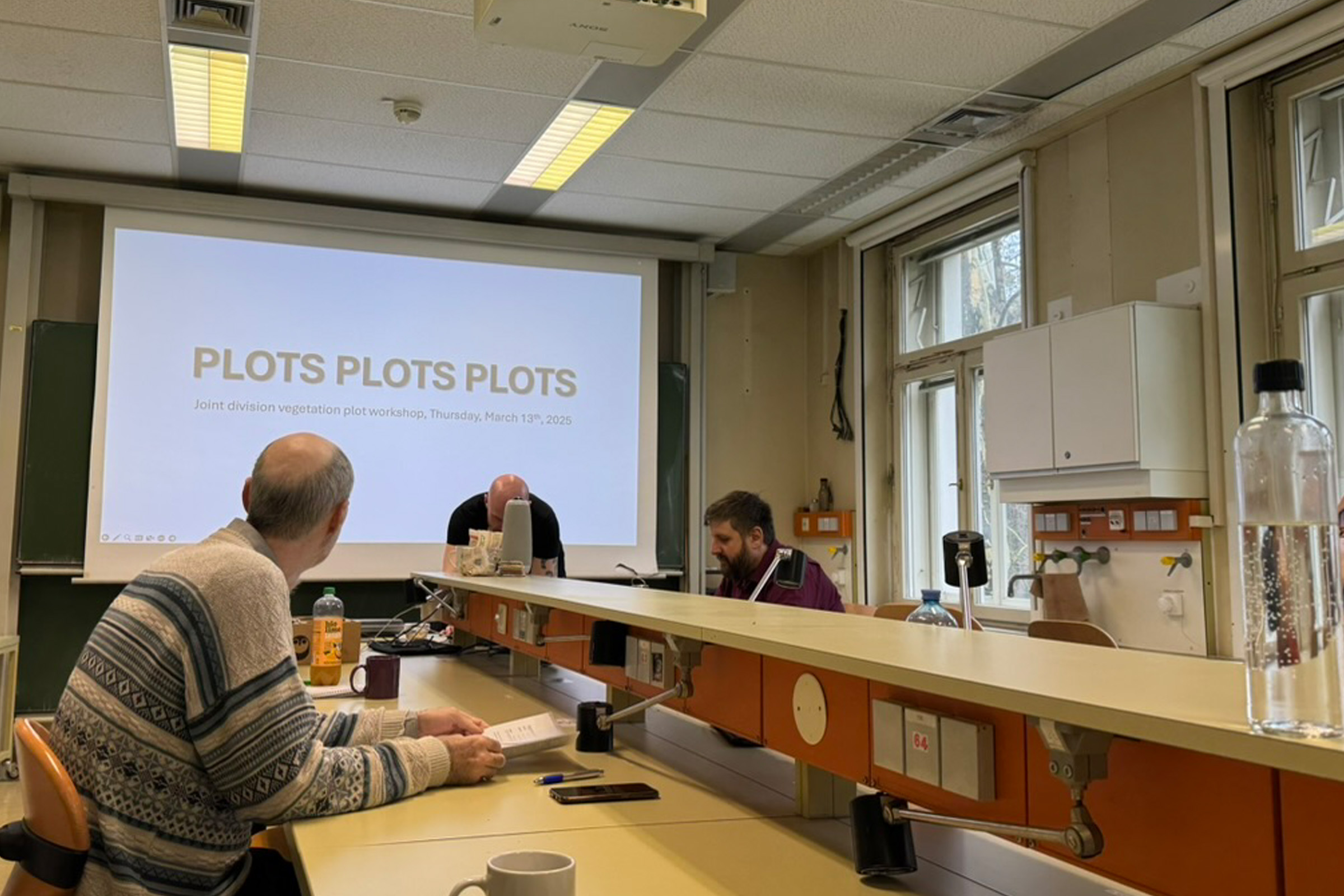
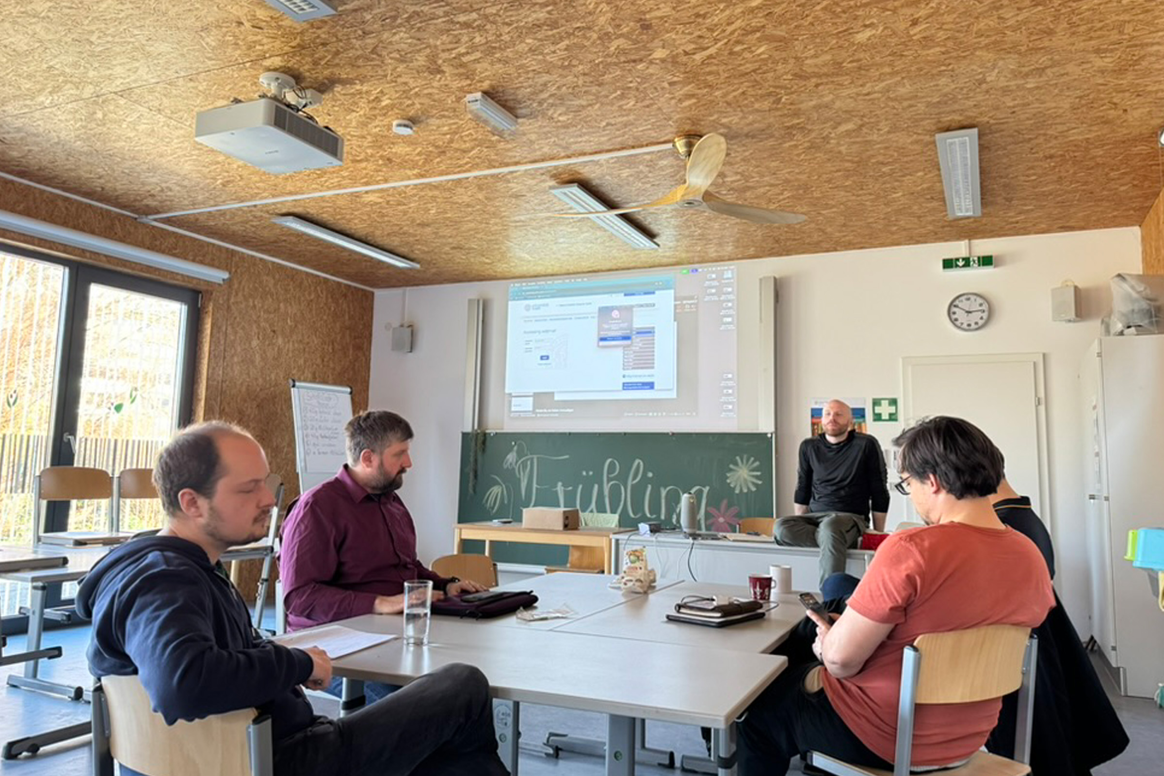
EducationThe Vegetation Plot Data Workshop took place at the Department at Rennweg, bringing together in house researchers working with vegetation plot data to discuss shared challenges and develop a more efficient and reproducible workflow. Organized by Michael Glaser and Bernd Lenzner, the one-day workshop provided an informal and interactive space to exchange experiences, identify common hurdles, and explore solutions for handling, standardizing, and analyzing plot data.
Take aways
We chose three common struggles when working with plot based data: data cleaning and standardization, taxonomic harmonization, and linking to other data sources. As for the output of the workshop: we made a table for common data sources and tools people want to combine with their plot data and additionally a table of common issues and pitfalls and suggestions on how to tackle these issues.
More generally we had a discussion about a checklist of common errors, such as duplicate plots and different abundance scales. Maybe this can be followed up with a short paper on how to deal with large plot databases.
Morning
A short round of introductions
Many of us work with plot data, yet we often do so in isolation, reinventing the wheel rather than building on existing solutions. This became clear during a recent workshop where researchers from different backgrounds shared their experiences with plot data and its challenges, pitfalls, and best practices. Long-time experts and newcomers, everyone at the workshop had his own perspective on working with plot data
Michael has been working with EVA and resurvey data for years and has the experience to handle many challenges.
Andy encounters plot data occasionally and is interested in workflow best practices, though data format inconsistencies remain a hurdle.
Bernd has limited experience but is now involved in projects that rely on plot data, making it important to understand its challenges.
Me (Gilles) sees over- and under-sampling as the biggest hurdles when working with plot data.
Ekin struggles with understanding column definitions and what they actually represent but plans to rely on colleagues like Michael and Joni to overcome these issues.
Wolfgang works extensively with relevees, contributing to the Austrian Vegetation Database (75,000 relevees) and EVA. Managing this data optimally would be a full-time job, but he does it in his spare time. Missing coordinates, incomplete records, and taxonomic standardization are major bottlenecks.
Joni builds species distribution models (SDMs) using EVA data but finds taxonomic harmonization a persistent issue. EVA is not fully harmonized, requiring manual checks with external sources like POWO.
Daijun has used forest plot data since his PhD and plans to work with sPlot data in the future. Geographic bias and inconsistencies in plot size remain challenges.
Elias is just beginning to compile and format plot data for his PhD, finding the process of preparing data to be a major hurdle.
Karl has worked with plot data to varying degrees of success. Data quality and distribution issues have sometimes been insurmountable, leading him to circumvent rather than resolve certain challenges.
Results of the questionaire
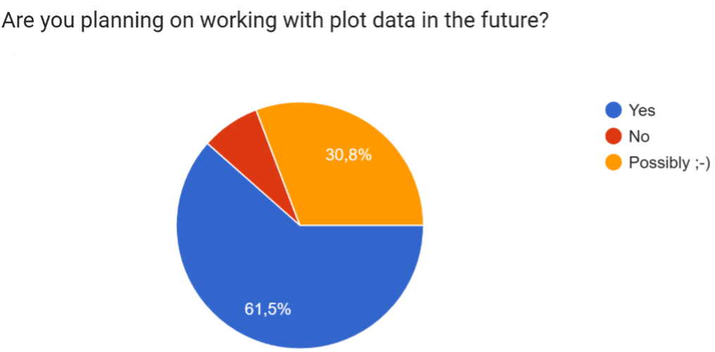
The majority of respondents (61.5%) plan to work with plot data in the future, with a smaller portion uncertain (30.8%) and only one person indicating they won’t. This confirms that plot data will remain an important component for our group, making discussions around best practices still relevant.
In the survey, participants ranked common challenges in working with plot data. After applying some fancy math*, we came up with the following ranking:
Data cleaning
Reproducible reports
Taxonomic harmonization
Linking to other data sources
Metadata issues and feedback
Plot level metrics
*The ranking was calculated using Likert scaling, where topics were scored from -3 (not relevant) to +3 (highly relevant) and weighted by the number of votes. Other ranking methods produced similar results, reinforcing these as priority areas for the community. Ultimately, people can decide what they find relevant.
Forming break out groups
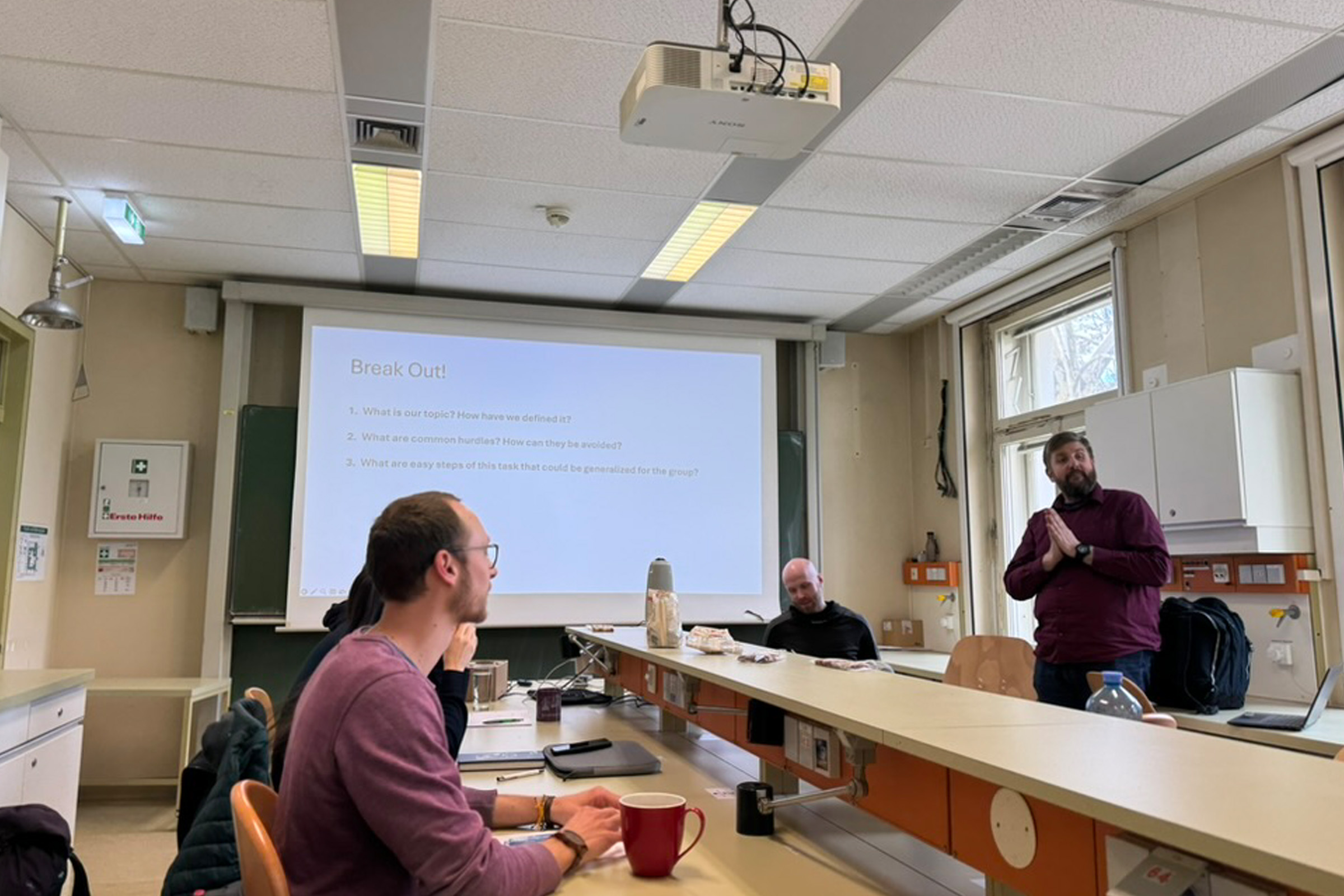
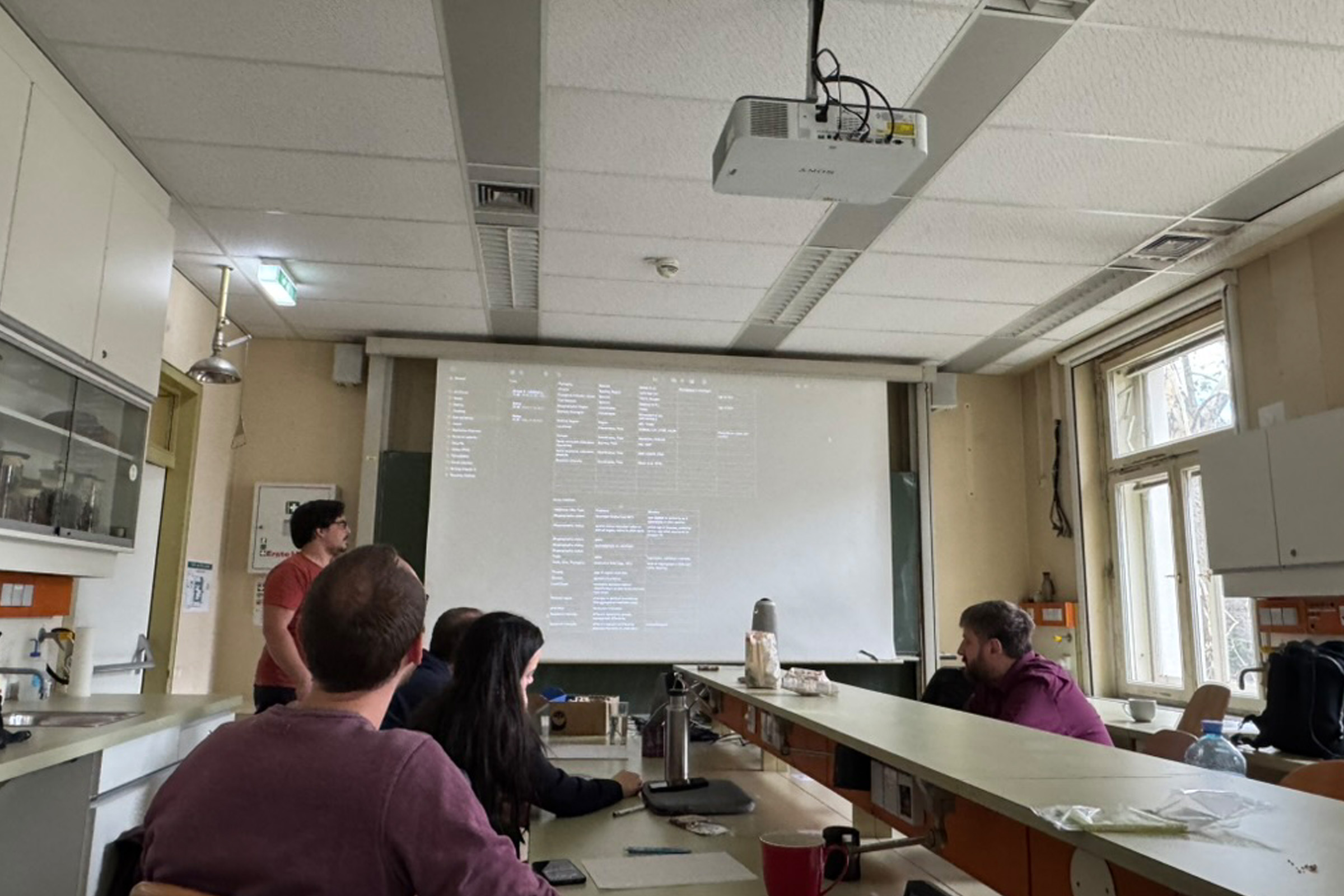
During the morning breakout session, we split into three groups to focus on topics 1,3 and 4 as these gathered the most interest. Each group discussed common challenges, shared experiences, and possible solutions. The output should be a sharable document to be used by new people or people already working with the data as a guidline.
Group 1: Topic 1 - Data cleaning (and beyond)
Participants: Andi, Elias, Karl (+Emma joining later)
Group 1 focused on data cleaning and standardization, though the discussion extended to broader topics. They identified the need for a unified format for data analysis, as inconsistencies persist even within the same project. Terms like Taxon, Species, and PlantName are not always used consistently, highlighting a necessity of establishing project-wide and department-wide standards, ideally with some level of automation or data standards everyone should follow.
Karl has a personal list of data sources that he considers when starting new projects, which could be useful for others as well. The group discussed how different sources are used inconsistently across projects and how a more unified approach could improve data handling. They also explored how to integrate data into department-wide standards and debated naming conventions for plot IDs, weighing the benefits of composite vs. free-standing primary keys and the need to define a normal form for structuring data. As the discussion got sidetracked they tried to refocus by working backward from the goal of what they want.
The group saw value in creating checklists and workflows, potentially including code snippets, but saw challenges in how to store, share, and especially maintain these resources to keep them up to date. While the discussion was not highly structured, important points were raised.
Group 2: Topic 3 - Taxonomic standardization
Participants: Joni, Ekin, Wolfgang
The group discussed the challenges of taxonomic harmonization and how to approach it effectively. One key takeaway was the importance of clarifying needs before starting:
Small-scale studies → Manual verification may be manageable.
Large-scale datasets → Automation is necessary
They also considered the scope of harmonization, emphasizing the need to avoid unnecessary complexity. A major question that should always be asked is whether subspecies and varieties need to be included, as this can significantly increase the workload. These are the main R packages people are using:
WFO (World Flora Online) is the main reference people are using right now
rWCVP (Royal Botanic Gardens, Kew’s World Checklist of Vascular Plants)
taxize (allows macthing across multiple sources, including WFO, GBIF, and ITIS)
The group noted that The Plant List has been discontinued, requiring users to rely on more current tools. But also with these tools challenges remain. One such issue is fuzzy matching, which is not always reliable and should be used cautiously. Difficulties also arise when standardizing aggregates, varieties, and hybrids, as they do not always fit neatly into existing frameworks. The group suggested that a list of known issues could help prevent recurring problems and provide clearer guidelines for future users.
Group 3: Topic 4 - Linking to other Data Sources
Participants: Gilles (me), Daijun, Michi, Bernd
My group focused on the challenges and strategies for integrating external data sources into plot-based research. We discussed how different datasets can be linked, common pitfalls, and potential solutions. We came up with a table to summarize the information:
Data sources:
| Type | Connection | Sources | Tools |
|---|---|---|---|
| Biogeographic status | Species, Region | GloNAF , GIFT , POWO , Kalusová et al. (2024) | DASCO , bRacatus (R packages) |
| Traits | Species | TRY , GIFT , BIEN , GRooT , WCUPS | |
| Phylogeny | Species | Qiang & Jin (2016) | PhyloMaker (R package) |
| Threats | Species, Region | IUCN Red List | |
| Ecological Indicator values | Species | Tichý et al. (2023) , Dengler et al. (2023) | |
| First Records | Species | Seebens et al. (2023) | |
| Biogeographic Region | Coordinates | TDWG | |
| Biomes / Ecoregion | Coordinates | TEOW (Olson et al., 2001), Global Ecoregions (Dinerstein et al., 2017), Anthromes (Ellis et al., 2010) | |
| Political Region | Region | ISO , TDWG | |
| Landcover | Coordinates, Time | CORINE , LUH , HYDE , HILDA+ | |
| Climate | Coordinates, Time | WorldClim , CHELSA | |
| Socio-economic indicators (countries) | Country, Time | HDI , GDP | |
| Socio-economic indicators (explicit) | Coordinates, Time | GDP , HANPP , OSM | |
| Research Intensity | Coordinates, Time | Meyer et al. 2015 |
Afternoon
Breakout Group Discussions
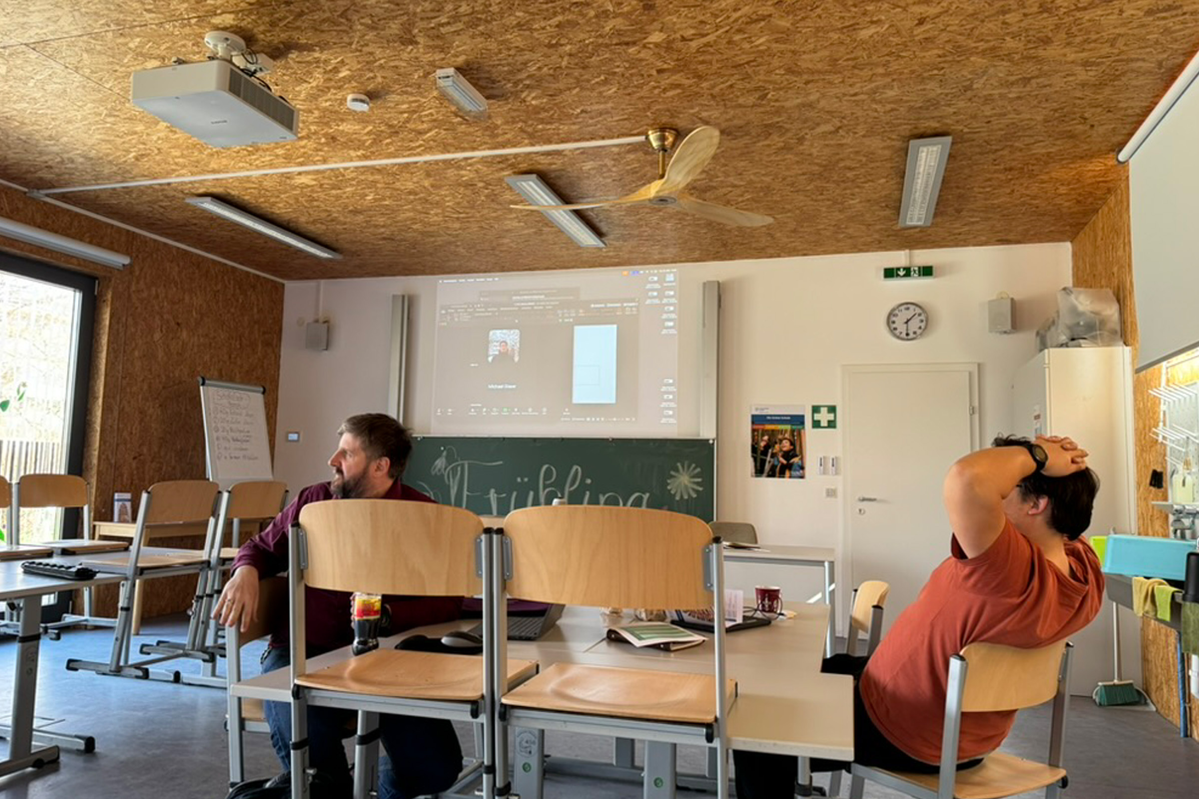
In the afternoon, Groups 1 and 2 combined to continue their general discussions on guidelines for handling plot data. Group 3 focused on improving the framework for linking external data sources, with Ekin joining the discussion. The shift in structure aimed to refine the morning's ideas. Group 3 continued their work on the tables and Group 1 & 2 had some issues to define a clear outcome, leading to a more open-ended discussion.
Group 1 & 2: Defining Common Guidelines
Participants: Joni, Ekin, Wolfgang, Andi, Karl, Emma, Elias
The merged group explored different aspects of data standardization and taxonomic harmonization, leading to a broad discussion of recurring challenges. They started a table listing common issues encountered when working with large plot datasets, including:
Duplicate plots
Differences in abundance scales
Other known inconsistencies that can impact data integrity
The idea of a checklist of common errors was voiced. This should be available to the whole department.
Group 3: Expanding Linking Data Sources
Participants: Ekin, Bernd, Michi, Gilles (me)
My group continued refining the approach to linking external data sources. We identified two main categories of problems:
Limitations of the data itself (e.g., missing information, outdated classifications).
Challenges in linking different sources (e.g., inconsistencies in geographic or taxonomic definitions).
They discussed sharing the table as an online document for broader accessibility, potentially integrating it into the BioInvasion Wiki to serve as a community resource. The table was structured into two parts 1) A table of data sources (which datasets to use for specific attributes) and 2) A table of issues (common pitfalls and how to address them).
Limitations and Resolutions:
| Type | Limitations of Data | Limitations of Linking Data | Approach to Address These Limitations |
|---|---|---|---|
| Biogeographic status | Mismatch GloNaf and GIFT | Use GloNAF as the authority for alien species classification since it specializes in alien species. | |
| Spatial status mismatch (alien in part of region, native in other part) | Cross-check the age and source of biogeographic data. Use multiple sources as a tie-breaker (e.g., regional floras, expert assessments). | ||
| Data Gaps | Use complementary sources (e.g., national databases, regional species checklists) to fill gaps. | ||
| Classifying archaeophytes vs. neophytes | |||
| Climate* | Spatial uncertainty in climate datasets | ||
| Extreme years in climate records | Apply rolling averages (e.g., past 10–30 years) to smooth outlier years | ||
| Broad range of available future climate projections | Use multiple global circulation models (GCMs), including region-specific models, and ensemble averaging to capture projection uncertainties. | ||
| First Records | Resolution is often at the country level (adequate for continental but not fine-scale analyses) | Infer finer-scale estimates using surrounding country data, species’ median residence times, or expert-verified local records. | |
| Uncertainty in first record data (earliest record ≠ actual first establishment) | Validate with additional sources (e.g., GBIF occurrence data, herbarium records) and apply probabilistic approaches to estimate introduction timing. | ||
| Land Cover* | Mismatch between plot-level habitat classification and land cover datasets | ||
| Accounting for gross vs. net land use change (e.g., what changes to what) | Track specific land use transitions over time | ||
| Political region | Changes in political boundaries affecting spatial data | Apply standardized disaggregation methods for boundary changes or use historical boundaries when necessary. | |
| Research intensity | Uneven representation of taxonomic groups | Apply sampling corrections (e.g., rarefaction) and account for taxonomic biases in analysis. | |
| Uneven regional contributions to datasets | Use methodological controls (e.g., weighting by sampling effort) and acknowledge source biases. | ||
| Socio-economic data (countries) | Differences in socio-economic indicator definitions between countries and across time | Harmonize indicators by aligning definitions and adjusting for temporal shifts. | |
| Socio-economic data (explicit indicators) * | Incomplete reporting or gaps in indicator-specific data | Use interpolation cautiously; validate interpolated values with alternative socio-economic datasets. | |
| Threats | Outdated region-level species lists | ||
| Traits | Data Gaps | Impute missing trait values based on phylogenetic or ecological similarity. Validate imputed values and consider using CSR mapping instead | |
| Differences in measurement source (e.g., in situ vs. lab; different life stages; native vs. invaded ranges; experimental vs. natural conditions) | |||
| Environmental plasticity in trait expression | Use summary statistics (minimum, maximum, average) and analyze the range width to capture variability for robust comparisons. | ||
| Traits, EIVs, Phylogeny | Taxonomic resolution differences (e.g., subspecies vs. varieties) | Harmonize taxonomic levels when integrating data |
*Considerations for Grid-Based Data
| Limitations | Solutions |
|---|---|
| Inconsistent spatial and temporal resolutions | Apply appropriate downscaling or upscaling techniques carfully |
Reflections on the Workshop
The workshop was a good effort in sharing common struggles and ideas. I liked the six topics we focused on. They covered most issues people face when working with plot data. There was, however, concern from people about where this would be shared. Without knowing where the outputs would go, some people were unsure what the outcome of the discussions would be.
That was especially noticeable in the afternoon session. Some lacked concrete goals, and without a clear output, discussions drifted. Having something specific (i.e a Word document, a structured table or a checklist) could have helped keep things more focused. Since I am not formally trained in ecology or even biology, I found the list of challenges and solutions really useful. It is not just relevant internally but could also help new PhD or master's students who are starting to work with plot data.
If I had one suggestion, it would have been good to have a clear output goal from the start. Otherwise, people just discuss and not much happens afterward. Bernd had a good idea of following up with a paper on dealing with plot data, perhaps something like "10 Common Pitfalls." That could be a good next step.