Simulate data from ratio models

Generate simulated datasets from prior or posterior predictive distributions. Useful for prior predictive checks, simulation-based calibration, and understanding model behavior.

Usage

sim_ratiod(
  n = 100,
  family = ratiod_negbin_negbin(),
  formula = NULL,
  beta_num = NULL,
  beta_denom = NULL,
  sigma_re = 0.5,
  phi_num = 5,
  phi_denom = 5,
  n_groups = 10,
  n_per_group = NULL,
  spatial = NULL,
  seed = NULL
)

Arguments

n

Number of observations to simulate.

family

A tulpaRatio family object specifying the distributions.

formula

Optional formula for generating covariates and structure. If NULL, generates intercept-only data.

beta_num

Numeric vector of true numerator coefficients. If NULL, drawn from prior.

beta_denom

Numeric vector of true denominator coefficients. If NULL, drawn from prior.

sigma_re

Standard deviation of random effects. Default 0.5.

phi_num

Overdispersion for numerator (negbin/gamma families). Default 5.

phi_denom

Overdispersion for denominator (negbin/gamma families). Default 5.

n_groups

Number of random effect groups. Default 10.

n_per_group

Observations per group. If NULL, groups are unbalanced.

spatial

Optional spatial structure specification.

seed

Random seed for reproducibility.

Value

A list with class ratiod_simdata containing:

data

Data frame with simulated observations

true_params

List of true parameter values used

family

Family specification

n

Number of observations

Details

The simulation generates data according to the ratio model structure:

For negbin_negbin:

• y_num ~ NegBin(mu_num, phi_num)

• y_denom ~ NegBin(mu_denom, phi_denom)

• log(mu_num) = X %*% beta_num + re

• log(mu_denom) = X %*% beta_denom + re (shared RE)

For binomial:

• y_num ~ Binomial(y_denom, p)

• logit(p) = X %*% beta + re

For poisson_gamma:

• y_num ~ Poisson(mu_num)

• y_denom ~ Gamma(shape, rate) where rate = shape / mu_denom

See also

tratio() for model fitting, prior_predict() for prior checks

Examples

# Simulate CPUE-type data
sim <- sim_ratiod(
  n = 200,
  family = ratiod_poisson_gamma(),
  beta_num = c(2, 0.5),      # intercept + depth effect
  beta_denom = c(1, 0.2),    # effort model
  sigma_re = 0.3,
  n_groups = 20,
  seed = 123
)

# View simulated data
head(sim$data)
#>   y_num  y_denom         x1 x2 group
#> 1    13 3.415682  2.1284519  1    15
#> 2     7 3.161744 -0.7413361  0    19
#> 3     3 3.380566 -1.0959963  1    14
#> 4     6 1.117076  0.0377884  1     3
#> 5    13 1.886051  0.3104807  0    10
#> 6     9 3.979671  0.4365235  0    18

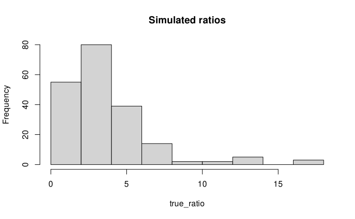
# Check true ratio distribution
true_ratio <- sim$data$y_num / sim$data$y_denom
hist(true_ratio, main = "Simulated ratios")


# Simulate binomial proportion data
sim_binom <- sim_ratiod(
  n = 100,
  family = ratiod_binomial(),
  beta_num = c(-0.5, 1),     # logit-scale coefficients
  n_groups = 10,
  seed = 456
)

# \donttest{
# Fit model to simulated data (slow, not run on CRAN)
fit <- tratio(
  y_num | y_denom ~ x1 + (1 | group),
  data = sim$data,
  family = ratiod_poisson_gamma(),
  control = list(iter = 200, warmup = 100, chains = 1)
)
#> Inference: Exact (Tier 1)
#>   Backend: hmc
#>   Reason: default (full MCMC)
#> Fitting ratio model...
#>   Family: poisson_gamma
#>   Observations: 200
#>   Iterations: 200 (warmup: 100)
#> Running NUTS sampler...
#>   Parameters: 26
#>   Iterations: 200 (warmup: 100)
#>   Chains: 1 (cores: 1)
# Compare estimated vs. true parameters
# summary(fit)
# sim$true_params
# }